The Search Evaluation Catalog
The measurement discipline: NDCG, MAP, MRR, judgment collection, online vs offline, A/B testing, regression detection.
About This Catalog
This is Volume 5 of the Search Engineering Series, covering search evaluation — the discipline of measuring search quality and using those measurements to drive improvement. Where Volume 1 documented query-time architectural patterns and assumed the reader could measure whether those patterns produced good results, this volume covers the measurement side: what metrics matter, how to collect the data they need, what evaluation modes (offline judgment lists, A/B tests, interleaving) fit which decisions, and how to run the continuous evaluation loop that keeps production search quality from eroding silently.
Search evaluation has historically been the most underdeveloped part of search engineering practice. Many production search teams ship features without measuring whether they help. Many search vendors sell platforms without telling customers how to know if the platform is working. The accumulated practitioner discipline exists in scattered form — textbooks (Manning et al., Grainger, Turnbull), academic literature on metric design and counterfactual evaluation, vendor documentation on A/B testing infrastructure, conference talks at Haystack and SIGIR — but it hasn't been consolidated into Fowler-style structural reference. This volume aims to fill that gap.
The volume's perspective. Evaluation is engineering practice, not a one-time setup. The most important pattern in this volume isn't any individual metric or method — it's the continuous evaluation loop (Chapter 5) that integrates the others. Production search teams that take evaluation seriously do it weekly or daily; teams that treat it as a quarterly exercise see their search quality drift in ways they can't diagnose. The volume's individual patterns matter, but the discipline of using them together as ongoing practice matters more.
Scope
Coverage:
- The offline-online evaluation spectrum: static judgment lists, offline log replay, shadow deployment, A/B testing, interleaving.
- The metrics landscape: NDCG (the dominant metric), MAP, MRR, P@K, ERR, and the cases each fits.
- Judgment collection: explicit expert labeling, crowdsourced annotation, implicit signals from production, LLM-as-judge.
- Online evaluation: A/B testing methodology for search, interleaving (TDI and successors), bandit methods.
- Click modeling and counterfactual evaluation: handling position bias and presentation bias in production data.
- Regression detection: golden query sets, continuous evaluation, alert design for search quality.
- The evaluation-tuning loop: how evaluation feeds tuning and how tuning feeds back into evaluation.
Out of scope (covered in other volumes):
- Query-time architectural patterns (BM25, dense retrieval, hybrid, cascade). Volume 1 covers.
- Query understanding patterns (tokenization, normalization, intent classification). Planned Volume 2.
- Indexing and document engineering. Planned Volume 3.
- Ranking algorithms in depth (LTR feature engineering, training methodology). Planned Volume 4.
- Day-to-day tuning operations (query log analysis workflows, zero-result handling). Planned Volume 6 (Search Operations).
- Search UX evaluation specifically. Planned Volume 7 (Search UX Patterns) covers UX patterns; this volume covers their evaluation.
How to read this catalog
Part 1 ("The Narratives") is conceptual orientation: why search evaluation differs from general ML evaluation; the offline-online spectrum that organizes the methods; the metrics landscape and what each metric measures; judgment collection as the foundational discipline; the evaluation-tuning loop that integrates the rest. Five diagrams sit in Part 1.
Part 2 ("The Substrates") is the pattern reference, organized by section. Each section opens with a short essay on what its patterns share. Representative patterns appear in the Fowler-style template established by the agentic AI catalog and continued in Volume 1 of the search series.
Part 1 — The Narratives
Five short essays orient the reader to search evaluation as engineering discipline. The reference entries in Part 2 assume the vocabulary established here.
Chapter 1. Why Search Evaluation Is Different
Search evaluation borrows from general machine learning evaluation, from web product analytics, and from information retrieval academic literature, but it isn't any of these. Practitioners coming from adjacent fields often try to apply their familiar evaluation patterns and find that they don't quite fit. Understanding the specific shape of search evaluation — what makes it different from these adjacent disciplines — is the prerequisite for understanding why the patterns in this catalog look the way they do.
Search evaluation differs from general supervised ML evaluation in three ways. First, the labels are sparse and expensive: for a given query, only a small fraction of the corpus is judged, and the judgments require human relevance assessment that doesn't scale like other annotation tasks. Second, the metrics are position-sensitive: a relevant document at position 1 is worth more than the same document at position 10, in a way that classification accuracy doesn't capture. Third, the production signal is heavily biased: click data is shaped by what users were shown, which means naive aggregation produces self-reinforcing failure modes (the system promotes what users clicked, users click what was promoted, repeat). These three features — sparse labels, position sensitivity, biased production signal — require evaluation methodology that general ML evaluation doesn't provide out of the box.
Search evaluation differs from general web product analytics in two ways. First, the unit of evaluation is the query-result interaction, not the user session or the page view. A user issues multiple queries per session; each query is its own search engagement; evaluation needs to handle the per-query unit. Second, the relevant outcome isn't "engagement" in the social media sense but "found what they were looking for" — which sometimes means the user clicks one result and leaves the system (success), sometimes means the user clicks many results without finding what they wanted (failure), sometimes means the user doesn't click anything and gives up (clear failure). Standard product analytics tracks the wrong signals if applied naively.
Search evaluation differs from academic IR evaluation in two ways. Academic IR has produced foundational metrics (NDCG, MAP, MRR), benchmark collections (TREC, BEIR, MS MARCO), and evaluation methodology that production teams should and do borrow from. But academic evaluation operates on relatively stable corpora with carefully constructed judgment sets, while production search has continuously changing corpora, queries the academic test sets don't cover, and operational constraints that academic methodology doesn't address. The gap between academic IR and production practice is real and productive — academic literature provides the methodological foundation; production practice provides the operational reality. Search evaluation as documented in this volume sits in the gap.
The volume's approach reflects this hybrid position. The metrics (Section B) come substantially from academic literature; the patterns for using them in production (Sections A, D, E, F, G) are practitioner discipline. The methodology cited throughout draws from both sources because production search evaluation needs both: foundational metrics that academic literature established and refined, plus practitioner patterns for collecting data, handling biases, and integrating evaluation into engineering workflow that academic work doesn't cover.
Chapter 2. The Offline–Online Spectrum
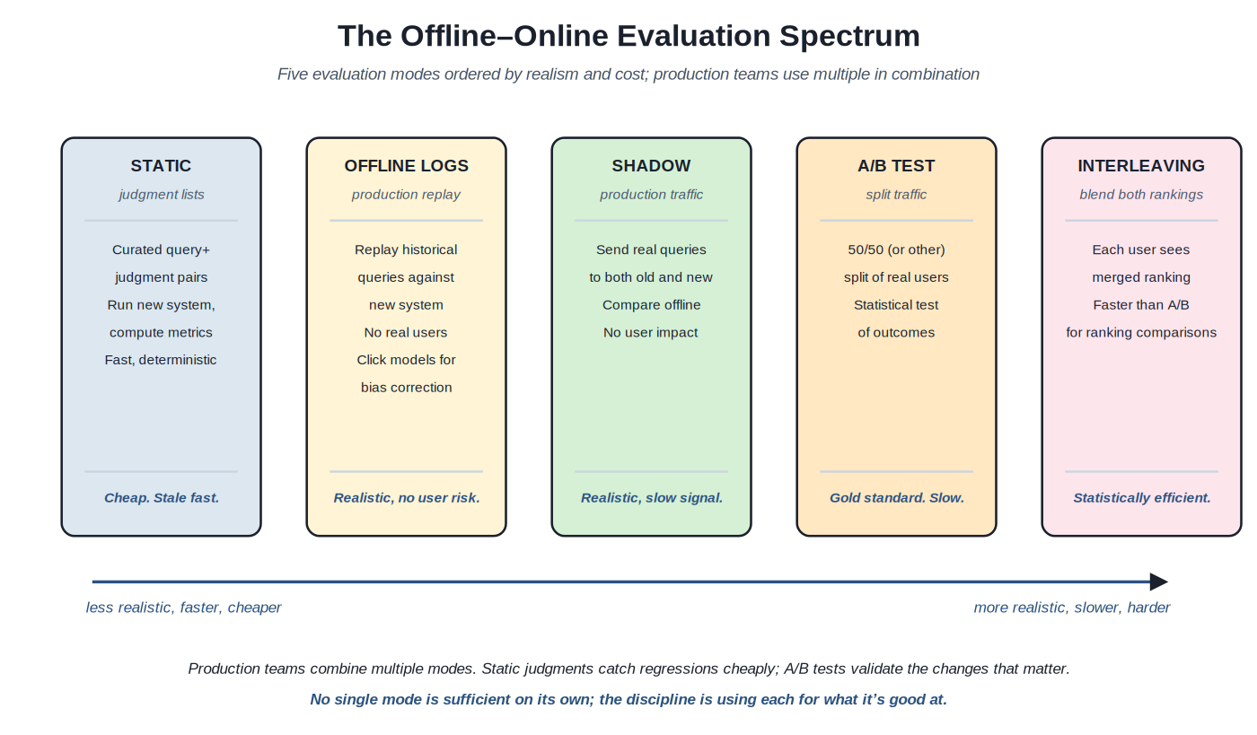
Search evaluation modes fall on a spectrum from purely offline (static judgment lists evaluated without user involvement) to purely online (production traffic split between systems). Each mode has characteristic strengths and limitations; production teams typically use multiple modes in combination. Understanding the spectrum — what each mode is good at, what it misses, what it costs — is the framework for choosing which evaluation to apply to which decision.
Five evaluation modes ordered by realism and cost. Production teams use multiple modes in combination; no single mode is sufficient.
Static evaluation uses curated judgment lists: query-document pairs with human-assigned relevance grades. To evaluate a system, you run the queries against it and compute metrics from the relevance grades of the returned documents. The mode is fast (no users involved, deterministic), cheap (the judgments are reused across many evaluations), and supports rapid iteration. The mode's weakness is that judgment lists go stale: the corpus changes, the queries users actually issue evolve, the judgment definitions may not match current product requirements. Static evaluation is the foundation of search evaluation practice; teams without it can't evaluate anything cheaply. Teams that rely on it alone miss changes in user behavior the static set doesn't capture.
Offline log replay uses historical production data: queries actually issued by users, against either the documents that existed at the time or the current corpus, with metrics computed from production click logs (using click models from Section E to correct for biases). The mode is more realistic than static evaluation because the queries are real, but doesn't require putting real users at risk. The cost is significantly higher than static evaluation — each replay needs to actually run the queries against the system, generating data for the metric computation — but lower than online evaluation. Production teams use offline log replay for changes that need realistic query distribution but can't justify online experiment cost.
Shadow deployment sends real production queries to both the current system and a candidate new system, returning the current system's results to users while logging the candidate's results for offline analysis. The mode catches issues the new system has on real queries without risking user experience. The cost is operational (running two systems in parallel; both must scale to production query volume). The signal is slow to accumulate because no real user feedback on the candidate's results exists — evaluation depends on offline metrics computed against the logged candidate output, often using click models to predict what users would have clicked.
A/B testing is the gold standard for measuring whether a change improves outcomes. Half the users (or some other split) see the current system; the other half see the candidate; outcomes are compared statistically. A/B testing handles non-ranking changes (different UI, different result presentation, different filtering logic) that interleaving can't address. The cost is real: substantial user populations are needed to detect statistically significant effects; the experiment runs for days or weeks; users in the candidate arm may experience worse search (or better, but we don't know until it ends) for the experiment's duration. The discipline of A/B testing for search is itself substantial; Section D covers the methodology.
Interleaving (TDI — Team-Draft Interleaving — and its successors) blends two systems' rankings into a single result set shown to each user, then tracks which system's contributions get clicked. The mode is statistically more efficient than A/B testing for ranking comparisons: each user sees both systems' results and effectively serves as their own experiment, reducing the variance and the sample size needed. The mode's limitations: it only compares rankings (not non-ranking changes); it requires careful tie-breaking rules to handle documents both systems would have shown; the production engineering to implement it correctly is non-trivial. Production search teams that have implemented interleaving typically use it for fast ranking experiments and reserve A/B testing for changes the interleaving framework can't evaluate.
The combination pattern. Production search teams don't pick one mode and stick with it. The working pattern: static judgment evaluation in CI for catching regressions cheaply; offline log replay for changes that need realistic queries; A/B testing for system-level changes that affect outcomes; interleaving for fast ranking experiments. Each mode catches what the others miss; using them together produces an evaluation regime that catches more issues than any one mode could. The discipline isn't choosing the right mode — it's building an evaluation regime that uses the right combination of modes for the team's decisions.
Chapter 3. The Metrics Landscape
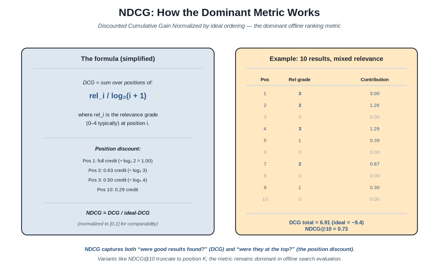
Search evaluation has multiple working metrics, each measuring something different about result quality. NDCG (Normalized Discounted Cumulative Gain) is the dominant metric in modern production practice; MAP (Mean Average Precision), MRR (Mean Reciprocal Rank), P@K (Precision at K), and ERR (Expected Reciprocal Rank) handle specific cases NDCG doesn't cover well. Custom business-aligned metrics (revenue per query, conversion rate, search-to-purchase) translate the academic metrics into business outcomes. Understanding what each metric measures — and what it doesn't — is the prerequisite for choosing the right metric for the decision.
NDCG captures both "were good results found?" (the gain) and "were they at the top?" (the position discount). The metric remains dominant in offline search evaluation.
NDCG's dominance comes from two properties. First, it handles graded relevance: rather than binary relevant/not-relevant, NDCG allows multiple grades (typically 0–4 or 0–5). A "highly relevant" result contributes more than a "somewhat relevant" result, matching the intuition that not all relevant results are equally good. Second, the position discount captures "relevance at the top matters more" in a principled way: the log₂(i+1) divisor means position 1 gets full credit, position 2 gets 63%, position 10 gets 29%, position 100 gets 15%. The discount is steep enough to reward high-quality top results substantially but gentle enough that documents at lower positions still contribute. NDCG's normalization (dividing by the ideal NDCG for that query) makes scores comparable across queries with different numbers of relevant documents.
MAP — Mean Average Precision — averages precision computed at every position where a relevant document appears, then averages across queries. MAP handles binary relevance (relevant or not) rather than graded. The metric is strong for queries where finding all relevant documents matters, not just the top few; legal search, scientific literature review, and similar use cases favor MAP. The metric is weaker than NDCG for typical web or e-commerce search where graded relevance and top-K focus matter more.
MRR — Mean Reciprocal Rank — takes the position of the first relevant result and averages 1/position across queries. The metric is tailored to known-item search and question-answering: "did we put the right answer at the top, and if not, how close?" Navigational queries ("nike air max", "apple support") are MRR-friendly. Discovery queries where users want to explore many results are MRR-hostile because MRR ignores everything past the first relevant result.
P@K — Precision at K — is the simplest metric: what fraction of the top K results are relevant? P@1, P@5, P@10 are common. The metric is intuitive (anyone can interpret "8 of the top 10 results were relevant") and tracks reasonable user experience for many search types. The metric ignores position within the top K (a relevant result at position 1 contributes the same as one at position 10) and ignores anything past K. P@K is often used alongside NDCG@K as an interpretable companion metric.
ERR — Expected Reciprocal Rank — models the user's likelihood of stopping at each result based on its relevance. The metric captures the idea that a highly relevant result early in the list "absorbs" the user's attention: they stop looking at subsequent results. ERR is more theoretically principled than NDCG but less widely adopted in production; teams using it typically have specific reasons (research-grounded relevance methodology) that justify the additional complexity.
Custom business metrics. Academic metrics measure relevance; business metrics measure outcomes. For e-commerce search, revenue per query, conversion rate, add-to-cart rate are common. For enterprise search, time-to-result, query-to-task-completion, repeat query rate measure productivity. For content search, click-through rate, dwell time, share rate measure engagement. The translation from academic metrics to business metrics is itself an evaluation discipline: a system that improves NDCG by 5% may or may not improve revenue by a measurable amount, and the relationship is workload-specific. Production teams typically track both academic and business metrics, with business metrics as the ultimate outcome and academic metrics as the proxy that supports rapid iteration.
The metric selection question. "Which metric should we use?" doesn't have a single answer. The metric should fit the decision being made and the use case being evaluated. For ranking changes evaluated offline against judgment lists, NDCG@10 is the typical default. For known-item search, MRR. For exhaustive retrieval (legal, scientific), MAP. For business decisions, the relevant business metric. Most production teams track multiple metrics in parallel; the discipline is interpreting them together rather than picking one to optimize.
Chapter 4. Judgment Collection
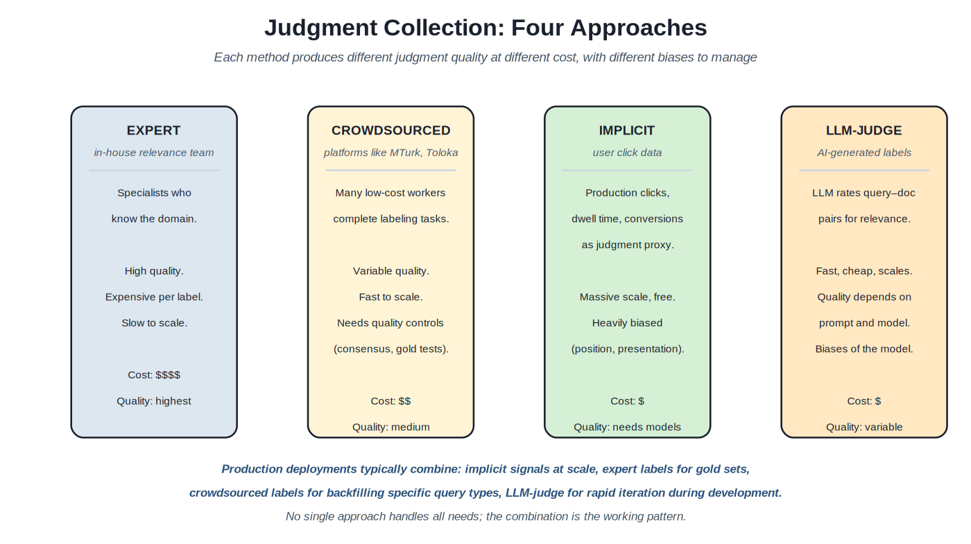
Every offline evaluation method needs judgments: assertions about which results are relevant to which queries. The judgment collection method shapes evaluation quality, cost, and what biases need handling. Four major approaches dominate: expert labeling (in-house specialists), crowdsourced labeling (commodity workers), implicit signals (production click data), and LLM-as-judge (AI-generated labels). Most production deployments use combinations; understanding the trade-offs is the prerequisite for designing the right combination.
Four approaches with different cost-quality trade-offs. Production deployments typically combine multiple approaches.
Expert labeling uses domain specialists — in-house relevance teams, search quality analysts, or external SMEs — to assign relevance grades to query-document pairs. The labels are high-quality because the assessors understand the domain, the relevance definition, and the edge cases. The cost is high: expert time is expensive; throughput is low (maybe 50–200 judgments per hour per assessor depending on complexity); scaling requires hiring and training more assessors. Expert labeling is the right choice for gold sets (small, high-quality judgment lists used to validate other judgment sources) and for high-stakes domains (legal, medical, regulated) where lower-quality judgments are unacceptable.
Crowdsourced labeling uses platforms like Amazon Mechanical Turk, Toloka, Appen, or Prolific to distribute labeling tasks to large numbers of low-cost workers. Throughput is high; cost per label is much lower than expert labeling. Quality is variable: individual workers produce noisy labels, but consensus across multiple workers per task produces reasonable quality. Quality controls (gold tests interspersed with real tasks; worker reputation tracking; consensus thresholds; explicit annotation guidelines) are essential. Crowdsourced labeling fits cases where significant judgment volume is needed and the relevance task is well-defined enough to explain to non-specialist workers.
Implicit signals use production click data as judgment proxy: documents that users click are treated as more relevant than documents they didn't click. The scale is enormous (millions of judgments daily for active production search), the cost is essentially free (the data is already being logged), and the signal is closer to user-perceived relevance than explicit labels. The trade-off is heavy bias: position bias (higher-ranked documents get more clicks regardless of relevance), presentation bias (results with rich snippets get clicked more), trust bias (results from known sources get clicked more). Section E covers click models and counterfactual evaluation — the methodology for extracting unbiased relevance signal from biased click data. Implicit signals are the right choice for evaluation at scale once the methodology for handling bias is in place.
LLM-as-judge uses large language models to assign relevance grades. Throughput is high; cost per label is low; the quality depends on prompt design and model capability. For some tasks, modern LLMs produce labels approaching expert quality. For others, they produce labels that look plausible but encode model biases that don't match the relevance definition the team intended. LLM-as-judge is emerging through 2024–2026 as a practical evaluation tool; the methodology is less mature than the other three approaches, and validation against expert gold sets is essential. The pattern is best for rapid iteration during development; production evaluation typically uses LLM-as-judge alongside (not instead of) other judgment sources.
The combination pattern. Production deployments rarely rely on one judgment source. The working pattern: expert labels for small high-quality gold sets used to validate everything else; crowdsourced labels for backfilling specific query types or domains where expert labels can't scale; implicit signals at production scale with click models for bias correction; LLM-as-judge for rapid iteration during development. Each source covers what the others miss; the combination produces evaluation that's scaleable, accurate, and adaptable to changing needs.
Chapter 5. The Evaluation–Tuning Loop
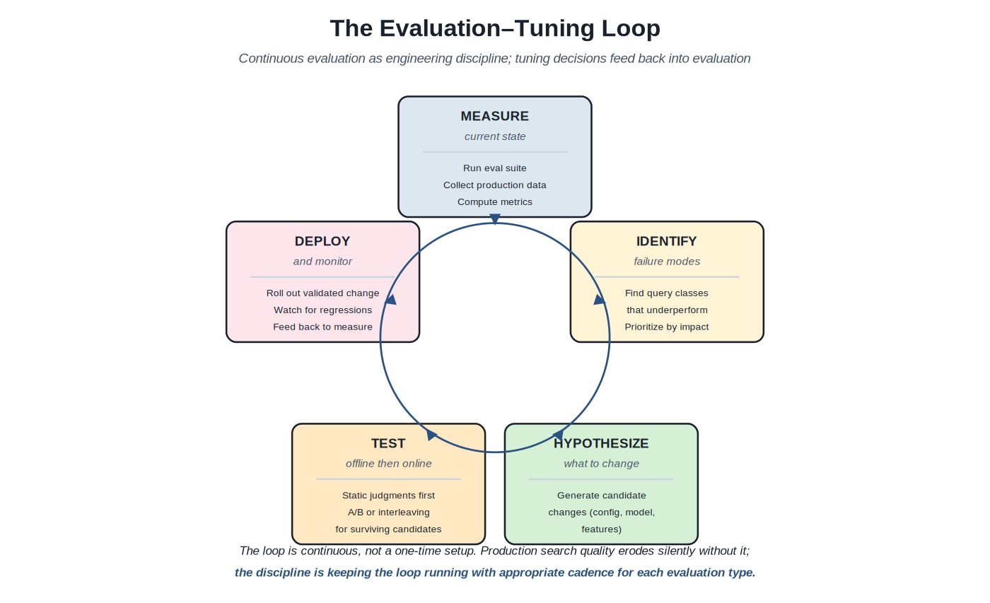
The most important pattern in search evaluation isn't any individual metric or method — it's the loop. Measurement that doesn't feed back into tuning is overhead; tuning that doesn't feed back into measurement is gambling. The continuous evaluation-tuning loop integrates the patterns documented elsewhere in this volume into ongoing engineering practice. Production teams that close the loop see their search quality improve; teams that treat evaluation as quarterly exercise see drift they can't diagnose.
Measure → identify → hypothesize → test → deploy → measure. Continuous, not one-time.
Measure. The first phase: run the evaluation suite against the current production system. Static evaluations against judgment lists produce metric scores. Production click logs produce implicit-signal-based metrics. A/B test results from in-flight experiments produce online metrics. The aggregate picture across all evaluation modes is what "measure" produces. Cadence matters: weekly or daily for active production systems; quarterly or annual for stable mature systems where rapid iteration isn't needed.
Identify. The second phase: find where the system is underperforming. Aggregate metrics tell you average quality; underperformance is typically concentrated in specific query classes. Long queries fail in characteristic ways; short queries fail differently. Specific intents (navigational, informational, conversational) have different failure modes. Specific user segments may experience worse quality than others. The discipline of identifying failure modes is itself substantial; the future Search Operations Catalog covers the analytics workflow.
Hypothesize. The third phase: generate candidate changes that might address the identified failure modes. Configuration changes (BM25 parameters, hybrid weights). Model changes (different embeddings, retrained LTR models). Feature changes (new ranking signals, new fields). UX changes (different result presentation). The hypothesizing phase is creative; the evaluation phase is critical. Hypothesizing without subsequent testing wastes engineering on changes that may not help; testing without hypothesizing produces no candidates.
Test. The fourth phase: evaluate the candidate changes. Start cheap: static evaluation against judgment lists catches obvious regressions. Move toward more realistic evaluation: offline log replay, then shadow deployment, then A/B testing or interleaving for the candidates that survive earlier filters. Most candidates fail at the cheap-evaluation stage; only the survivors deserve expensive online evaluation. The cascade structure (Chapter 4 of Volume 1 — cheap-and-many, expensive-and-few) applies to evaluation as much as to retrieval.
Deploy and monitor. The fifth phase: roll out validated changes to production. Gradual rollout (10% then 50% then 100%) with monitoring for regressions. The deployment isn't the end of the loop; it's the input to the next measurement cycle. Production behavior may differ from experiment behavior in ways the test didn't reveal; continued monitoring catches issues that emerge after deployment. The discipline of post-deployment monitoring is what closes the loop; without it, the loop is open and improvements don't compound.
Loop cadence. Different parts of the system warrant different cadences. Hot-path tuning (top queries, business-critical use cases): weekly or daily evaluation, monthly tuning cycles, quarterly model retraining. Long-tail tuning: monthly evaluation, quarterly tuning, annual or as-needed model retraining. Major architecture changes (Volume 1 patterns): quarterly or annual evaluation; the cost of evaluating architecture changes is high; the benefit of catching wrong architectural choices is also high. Production teams calibrate the cadence to the change rate and business impact of each part of the system.
The loop's relationship to organizational structure. Continuous evaluation requires named accountability: someone owns the metrics; someone owns the tuning; someone owns the deployment. Without ownership, the loop runs sporadically; with ownership, it runs continuously. Mature production search organizations typically have a search quality function (one or more relevance engineers, an analyst, sometimes a search product manager) whose job is the loop. The structural question — who owns search quality — is as important as the methodological question — what metrics and methods to use.
Part 2 — The Substrates
Eight sections cover the patterns and methods of search evaluation. Each section opens with a short essay on what its patterns share. Representative patterns appear in the Fowler-style template.
Sections at a glance
- Section A — Judgment list construction
- Section B — Offline metric patterns (NDCG, MAP, MRR, P@K)
- Section C — Judgment collection methods
- Section D — Online evaluation (A/B, interleaving)
- Section E — Click models and counterfactual evaluation
- Section F — Regression detection and continuous evaluation
- Section G — Custom business metrics
- Section H — Discovery and resources
Section A — Judgment list construction
The foundational artifact: queries with relevance judgments that drive everything else
Every offline evaluation depends on a judgment list: query-document pairs with assigned relevance grades. The construction of the list is a discipline in its own right. Naive construction (random queries, arbitrary judgments) produces noisy evaluations that hide real quality changes. Disciplined construction (representative queries, calibrated judgments, ongoing maintenance) produces evaluation infrastructure that earns its place across many tuning decisions.
Judgment list construction and pooling #
Source: TREC methodology (Voorhees, NIST); Manning et al., Introduction to Information Retrieval; Grainger, AI-Powered Search; OpenSource Connections methodology
Classification — The methodology for constructing the foundational judgment artifact — query selection, document pooling, judgment assignment.
Build a judgment list that supports reliable offline evaluation: representative queries that cover the production query distribution, document pools that capture the candidates any system might surface, judgments that are calibrated and reproducible across assessors.
A naive judgment list has predictable failure modes. Queries cherry-picked by the team don't reflect actual production traffic, so evaluation scores don't predict production quality. Documents judged are only those returned by the current system, so any candidate system surfacing different documents gets unfair scores (because the unjudged documents are treated as not-relevant by default). Judgments produced by a single assessor without calibration drift from any defensible relevance standard. The discipline of judgment list construction addresses these failure modes systematically.
Query sampling. The query list should reflect production traffic, not the team's intuitions about important queries. Sample from production query logs, stratified by query characteristics: head queries (high frequency, narrow set), torso queries (medium frequency, broader set), tail queries (low frequency, very diverse). A judgment list with only head queries misses the long-tail quality issues that drive user frustration. A typical production judgment list might have 200–500 queries spanning the frequency distribution.
Pooling. For each query, judgment lists need a pool of documents to judge. The naive approach — judge only what the current system returns — produces the bias described above. The TREC-style pooling approach: run multiple candidate systems against the query, take the top K from each, union the results, judge everything in the union. The pool includes documents the current system missed but candidates surface, eliminating the bias. Pool depth (K) typically 20–100; the deeper the pool, the better the evaluation supports systems that differ substantially from the baseline.
Relevance grading scale. The choice of scale shapes the judgment task. Binary (relevant / not relevant) is simple but loses information about how relevant. Graded scales (typically 0–4 or 0–5) capture more nuance but require clearer annotation guidelines. A common scale: 0 (not relevant), 1 (related but not what user wants), 2 (relevant), 3 (highly relevant), 4 (perfect match). The scale should match the relevance definition the team uses; consistency in interpretation matters more than the specific numeric range.
Annotation guidelines. Written guidelines explain what each grade means with concrete examples and edge cases. Without guidelines, different assessors interpret "relevant" differently and inter-annotator agreement is low. With guidelines, agreement is higher, judgments are reproducible, and disputes about specific judgments can be resolved by reference to the guideline. Annotation guideline development is itself a substantial discipline; production teams iterate on guidelines as edge cases are discovered.
Inter-annotator agreement. Measure how consistently different assessors grade the same query-document pairs. Common metrics: Cohen's kappa or weighted kappa for graded scales. Agreement scores below 0.6 suggest the annotation task or guidelines need work; scores above 0.8 are excellent. Low agreement means the judgment list is noisy; high agreement means it's reliable. Production teams typically maintain agreement targets and adjust guidelines when agreement drifts.
Maintenance. Judgment lists go stale. The corpus changes (new products, retired documents). User queries evolve (seasonal shifts, new terms). Production system changes alter what gets surfaced. A judgment list that worked well last quarter may not capture current quality concerns. Maintenance patterns: quarterly judgment refresh for active deployments; add new queries based on production trends; re-judge documents whose content changed; retire queries that no longer reflect current traffic.
Every production search team that does offline evaluation needs judgment lists. The investment is substantial but compounds across all subsequent tuning work; the alternative is each evaluation reinventing its own judgments. The pattern is foundational rather than optional.
Alternatives — pure online evaluation (A/B testing) for teams that can't justify judgment list investment but have enough traffic to support fast online experiments. LLM-as-judge (Section C) as a lower-cost approximation, with the caveats covered there. Most teams use judgment lists as the foundation and supplement with online evaluation; pure-online is rare in production search.
- Voorhees, "Variations in relevance judgments and the measurement of retrieval effectiveness" (TREC methodology, 1998)
- Manning, Raghavan, Schütze, Introduction to Information Retrieval, ch. 8 on evaluation
- Trey Grainger, AI-Powered Search, chapters on relevance judgment
- OpenSource Connections Quepid (quepid.com) for judgment list management
Code
// Example judgment list format (CSV)
// query, document_id, grade, judged_at, assessor_id
// Grade scale: 0=not relevant, 1=related, 2=relevant, 3=highly relevant

query,document_id,grade,judged_at,assessor
"running shoes",prod_12345,3,2026-04-15,assessor_01
"running shoes",prod_12346,2,2026-04-15,assessor_01
"running shoes",prod_12347,0,2026-04-15,assessor_01
"running shoes",prod_98765,3,2026-04-15,assessor_02
"trail running shoes",prod_12345,2,2026-04-15,assessor_01
"trail running shoes",prod_45678,3,2026-04-15,assessor_01

// Example pooling script (Python pseudocode)
def build_judgment_pool(queries, candidate_systems, pool_depth=20):
pool = defaultdict(set)
for query in queries:
for system in candidate_systems:
results = system.search(query, top_k=pool_depth)
for doc_id in results:
pool[query].add(doc_id)
return pool

// Example inter-annotator agreement check (Python)
from sklearn.metrics import cohen_kappa_score
agreement = cohen_kappa_score(
assessor_a_grades,
assessor_b_grades,
weights='quadratic' // for graded scales
)
print(f"Weighted kappa: {agreement:.3f}") // target > 0.6, ideally > 0.8
Section B — Offline metric patterns
NDCG, MAP, MRR, P@K — the metrics that turn judgment lists into evaluation scores
Chapter 3 of Part 1 covered the metrics landscape conceptually. This section documents the metrics as patterns: when each fits, how each is computed, what each catches and misses. The metrics work on top of judgment lists (Section A); without judgments, the metrics have nothing to compute.
NDCG and discounted gain metrics #
Source: Järvelin and Kekäläinen, "Cumulated gain-based evaluation of IR techniques" (ACM TOIS, 2002); ubiquitous in modern search evaluation
Classification — The dominant offline ranking metric — graded relevance combined with logarithmic position discount.
Score a ranked result list by combining the relevance grades of its results with a position discount that rewards relevant results appearing higher, normalized to enable comparison across queries with different ideal scores.
Search quality involves both "were good results found" and "were they at the top." Simpler metrics handle one or the other: precision-at-K handles "were good results found in the top K" but ignores position within the top K; reciprocal rank handles "where was the first good result" but ignores everything after. NDCG captures both dimensions in a single principled metric with graded relevance support, making it the default offline evaluation metric for modern search systems.
DCG computation. For a ranked result list, DCG (Discounted Cumulative Gain) sums the relevance gain at each position divided by a logarithmic position discount. The standard formula: DCG = sum over positions i of (rel_i / log₂(i + 1)), where rel_i is the relevance grade at position i. Position 1 gets full credit (divisor = log₂(2) = 1); position 2 gets 0.63 credit; position 10 gets 0.29; position 100 gets 0.15. The discount falls off but never reaches zero, so relevant documents anywhere in the list contribute.
Variant with exponential gain. Some implementations use 2^rel - 1 instead of rel directly, exponentially weighting high-grade results. The variant emphasizes finding highly-relevant documents over finding more moderately-relevant ones. The exponential variant is the original Järvelin-Kekäläinen formulation; the linear variant is also widely used. The choice affects scores but not relative rankings of systems on most workloads.
Normalization. Raw DCG isn't comparable across queries because queries with more relevant documents have higher possible DCG. NDCG normalizes by dividing by the ideal DCG (the DCG achieved by ranking all relevant documents in optimal order). NDCG = DCG / ideal-DCG produces scores in [0, 1] that are comparable across queries.
Truncation: NDCG@K. Most production evaluation uses NDCG@K — NDCG computed over only the top K positions. NDCG@10 is the most common variant: it reflects "quality of the first page of results" for typical search UX. NDCG@5 or NDCG@3 emphasize top-of-page even more. The truncation choice should match the use case; e-commerce typically uses NDCG@10 or NDCG@20; question-answering may use NDCG@3 or NDCG@5.
Aggregation across queries. The per-query NDCG scores are typically averaged across the query set to produce a single system score. Macro-averaging (mean of per-query scores) is the standard. Sometimes median or other robust statistics are used to reduce influence of outlier queries.
Limitations. NDCG depends on judgment quality — garbage in, garbage out. NDCG assumes the relevance grades are accurate; biased or noisy judgments produce biased or noisy NDCG. NDCG also doesn't directly measure user outcomes (click-through, conversion, revenue); it measures a proxy for relevance that correlates with outcomes but isn't identical to them. Production teams typically track NDCG alongside business metrics.
Default offline evaluation metric for ranking quality across most search use cases. Especially appropriate for e-commerce, web search, enterprise search, and content discovery where graded relevance and top-K focus both matter.
Alternatives — MRR for known-item search where only the first relevant result matters; MAP for exhaustive retrieval (legal, scientific); P@K for simpler interpretability; ERR for cases where user-stopping models matter. NDCG is the default; specific alternatives apply when their specific dimensions matter more.
- Järvelin and Kekäläinen, "Cumulated gain-based evaluation of IR techniques" (2002)
- Manning et al., Introduction to Information Retrieval, section 8.4
- Grainger, AI-Powered Search, chapters on evaluation
Code
// NDCG@K implementation (Python)
import math

def dcg(grades, k=None):
"""Compute DCG over a list of relevance grades (already in ranked order)."""
if k is not None:
grades = grades[:k]
return sum(
grade / math.log2(i + 2) # i+2 because i is 0-indexed; position is i+1
for i, grade in enumerate(grades)
)

def ndcg_at_k(grades, ideal_grades, k=10):
"""NDCG@K: DCG of actual ranking divided by DCG of ideal ranking."""
dcg_actual = dcg(grades, k=k)
dcg_ideal = dcg(sorted(ideal_grades, reverse=True), k=k)
return dcg_actual / dcg_ideal if dcg_ideal > 0 else 0.0

// Example usage with the judgment list from Section A
// Run the system, get document IDs in ranked order, look up grades:
query = "running shoes"
results = system.search(query, top_k=10) // returns ranked doc IDs
grades_in_results = [judgments[query].get(doc_id, 0) for doc_id in results]
all_grades_for_query = list(judgments[query].values())

score = ndcg_at_k(grades_in_results, all_grades_for_query, k=10)
print(f"NDCG@10 for '{query}': {score:.3f}")

// Aggregate across queries
import statistics
per_query_scores = [
ndcg_at_k(
[judgments[q].get(doc_id, 0) for doc_id in system.search(q, top_k=10)],
list(judgments[q].values()),
k=10
)
for q in test_queries
]
print(f"Mean NDCG@10: {statistics.mean(per_query_scores):.3f}")
print(f"Median NDCG@10: {statistics.median(per_query_scores):.3f}")
MAP, MRR, and P@K — the alternative offline metrics #
Source: Classical IR literature; Manning et al., Introduction to Information Retrieval; ubiquitous in evaluation tooling (trec_eval, ranx, pytrec_eval)
Classification — Alternative offline metrics that handle specific cases NDCG doesn't cover well.
Apply the right metric for cases where NDCG isn't the best fit: MRR for known-item search, MAP for exhaustive retrieval, P@K for simpler interpretability, ERR for user-stopping models.
NDCG is the default but isn't always the best fit. Known-item searches ("nike air max 270") want a metric that scores high if the right item is at the top and ignores everything else; NDCG's position-discount handles this but isn't as crisp as MRR. Exhaustive retrieval (legal documents, scientific papers, e-discovery) wants a metric that scores recall across all relevant documents; NDCG's position discount makes it less suited than MAP. Communication with non-technical stakeholders favors metrics that are intuitive; P@K ("8 of the top 10 were good") is more communicable than NDCG. The discipline is matching the metric to the use case rather than defaulting to one metric for everything.
MRR — Mean Reciprocal Rank. For each query, find the position of the first relevant result. Compute 1/position (1.0 for position 1, 0.5 for position 2, 0.1 for position 10, 0 if no relevant result in top K). Average across queries. The metric is tailored to known-item search: "did you put the right answer at the top, and if not, how close?" Strong for question-answering and navigational search. Weak for discovery queries where users want to explore multiple results.
MAP — Mean Average Precision. For each query, walk through the ranked results; at each position where a relevant document appears, compute the precision at that position (fraction of top-N results that are relevant for that N). Average these per-relevant-document precisions to get the Average Precision for that query. Mean across queries. The metric handles binary relevance and rewards systems that find all relevant documents, not just the top few. Strong for exhaustive retrieval (legal, scientific, e-discovery). Weak when graded relevance matters or when only top-K matters.
P@K — Precision at K. The fraction of the top K results that are relevant. Binary relevance (a document is relevant or not). Simple and interpretable. P@1, P@5, P@10 are common. Doesn't care about position within the top K; doesn't care about anything past K. Good for high-level communication; less informative than NDCG for detailed evaluation.
ERR — Expected Reciprocal Rank. Models user stopping behavior: the probability that a user stops at each position based on the result's relevance. A highly relevant result early in the list "absorbs" the user's attention; documents below it have lower expected impact. ERR is more theoretically principled than NDCG for modeling user behavior; less widely adopted because the marginal benefit over NDCG is small for most workloads and the additional complexity isn't justified.
Recall@K. The fraction of all relevant documents that appear in the top K. Used in retrieval evaluation (first-stage retrieval in cascade architectures, Volume 1 Section D) where the question is whether relevant documents make it into the candidate set, not their final ranking. Recall@100 or Recall@1000 are common for first-stage retrieval; recall in the candidate set bounds what the reranker can achieve.
When to use multiple. Production teams typically track multiple metrics in parallel: NDCG@10 as the headline offline metric; MRR for navigational query subsets; P@5 for stakeholder communication; Recall@100 for first-stage retrieval evaluation. Each metric catches what the others miss; using them together produces fuller evaluation than any one alone.
MRR: known-item search, question-answering, navigational queries. MAP: exhaustive retrieval, legal/scientific search, e-discovery. P@K: communication with non-technical stakeholders, top-of-page evaluation. ERR: research-grounded evaluation methodology, cases where the user-stopping model matters. Recall@K: first-stage retrieval evaluation in cascade architectures.
Alternatives — NDCG@K as the default for graded-relevance, top-K-focused use cases (most modern production search). The metrics in this entry are alternatives for specific cases; for general search evaluation, NDCG remains the default.
- Manning et al., Introduction to Information Retrieval, ch. 8
- Chapelle and Zhang, "Expected Reciprocal Rank for Graded Relevance" (CIKM 2009)
- trec_eval reference implementation (github.com/usnistgov/trec_eval)
- pytrec_eval / ranx Python implementations
Section C — Judgment collection methods
Explicit expert labeling, crowdsourcing, implicit signals, LLM-as-judge — the methods that populate judgment lists
Section A documented the construction of judgment lists structurally; this section documents the methods for actually collecting the judgments. Chapter 4 of Part 1 introduced the four approaches; this section makes them concrete patterns with operational details. The right combination depends on cost, scale, quality requirements, and the maturity of the search team.
Explicit expert labeling #
Source: Search relevance practitioner methodology; Quepid (OpenSource Connections); enterprise search teams at major e-commerce and content companies
Classification — Judgment collection by in-house specialists or trained domain experts who assign relevance grades according to annotation guidelines.
Produce high-quality relevance judgments by using assessors who understand the domain, the relevance definition, and the edge cases, accepting higher cost in exchange for higher quality.
Crowdsourced labels are cheap but noisy. Implicit signals are scaleable but biased. LLM-as-judge is fast but encodes model biases. For some uses — small gold sets validating other judgment sources, high-stakes domains where lower-quality judgments are unacceptable, calibration of annotation guidelines — the quality of expert labeling is necessary. Expert labeling can't scale to the volume that crowdsourcing handles, but for the cases that need it, nothing else substitutes.
Assessor selection. Domain expertise matters: e-commerce search assessors should understand the product domain; legal search assessors should understand legal relevance; healthcare assessors should have appropriate clinical knowledge. The assessors are typically in-house staff (search quality team, product specialists) or contracted SMEs (consultants, retired experts). Throughput is low — 50–200 judgments per hour per assessor depending on domain complexity — and cost is high (assessor time at SME rates).
Annotation tooling. Quepid (OpenSource Connections, free open-source) is the leading judgment management tool. The tool presents query-document pairs to assessors with the document content displayed; assessors assign grades with single-key input; the tool tracks assessor identity, timestamps, and inter-annotator agreement. Custom tools built on internal infrastructure are common for teams with specific requirements. The tool matters: a well-designed tool can double assessor throughput vs. a poorly-designed one.
Calibration sessions. Before independent labeling, assessors work through shared examples together, discussing edge cases and arriving at consistent interpretations of the relevance scale. The session produces calibration: assessors who have done this together agree more often than assessors who haven't. Recalibration sessions monthly or quarterly maintain agreement over time as new edge cases emerge.
Quality measurement. Inter-annotator agreement (Cohen's kappa or weighted kappa for graded scales) measures how consistently different assessors grade the same items. A subset of items is judged by multiple assessors to enable the measurement. Agreement scores below 0.6 trigger review of guidelines or recalibration; scores above 0.8 indicate the labeling task is well-defined and assessors are aligned.
Workload management. Expert assessors are expensive; their time should be used on the highest-value judgments. Patterns: judge new queries that production logs surface; judge query-document pairs near decision boundaries (where current and candidate systems disagree); judge the gold set used to validate other judgment sources; spot-check crowdsourced or LLM-judge outputs. Production teams typically have explicit workload prioritization.
Documentation. Maintain written annotation guidelines that capture the relevance definition, scale interpretation, edge cases, and decision rules. The guidelines are versioned; changes to guidelines may require re-judgment of affected items. The guidelines are the institutional knowledge of the search team's relevance discipline; without them, expert labeling doesn't survive assessor turnover.
Small gold sets (50–500 queries) used to validate other judgment sources. High-stakes domains (legal, medical, regulated) where lower-quality judgments are unacceptable. Calibration of annotation guidelines that other methods will follow. Edge cases requiring domain expertise to judge correctly. Annual or semi-annual high-quality evaluation that gold-standard methods support.
Alternatives — crowdsourced labeling for larger judgment volume at lower cost (next entry). Implicit signals for very large scale. LLM-as-judge for fast iteration. Expert labeling is the highest-quality method; the alternatives substitute for scale or cost reasons.
- Quepid (quepid.com / github.com/o19s/quepid) for judgment management
- OpenSource Connections methodology writings
- Trey Grainger, AI-Powered Search, chapters on relevance judgment workflow
Implicit signals and click-based judgments #
Source: Joachims et al. on click-based relevance learning (KDD 2002 and successors); production practice at all major web search and e-commerce companies
Classification — Using production click data, dwell time, and conversion signals as judgment proxy.
Extract relevance signal from production user behavior at scale, accepting that the signal is biased and requires modeling to interpret correctly, in exchange for judgment volume that explicit labeling can't produce.
Production search produces enormous volumes of user behavior data: queries, clicked results, dwell times on landing pages, conversions, abandoned searches. This data could in principle replace explicit judgment lists — it's real user signal at scale. The challenge: the data is heavily biased. Users click what was shown to them in the order it was shown; click data reinforces the current system's biases rather than measuring an external truth. Section E covers click models and counterfactual evaluation — the methodology for extracting unbiased relevance signal. This entry covers the patterns for collecting and using the raw signal.
Signals to log. Beyond clicks, production search should log: query text, time of query, user identifier (if available), what was shown (results, their positions, presentation features like rich snippets), what was clicked (which results, in what order), dwell time on each click (how long before user returned to results), subsequent actions (next query if reformulating; abandonment if leaving; conversion if purchasing or completing the task). The richer the logging, the more analyses become possible.
Click as relevance proxy. The simplest interpretation: clicked results are more relevant than non-clicked results. This works partially — users do tend to click what they find relevant — but with heavy bias: users click position 1 more than position 10 regardless of relevance; users click results with rich snippets more than plain ones; users click results from known brands more than unknown ones. Naive click-as-relevance produces self-reinforcing failure modes.
Dwell time. Users who click a result and stay on the landing page typically found something useful; users who click and immediately return (bounce) often didn't. Dwell time partially compensates for the click signal's noise: a click followed by long dwell is stronger evidence of relevance than a click followed by quick return. The pattern is sometimes called "satisfied click" vs. "unsatisfied click."
Conversion as ground truth. For e-commerce, the conversion (purchase) is the strongest relevance signal: users converted because they found what they wanted. For enterprise search, the analogous signal might be "task completed without further searches" or "result shared / forwarded." Conversion-based judgments are sparse (only a fraction of searches result in conversion) but strong; they're typically used alongside denser click-based judgments.
Query reformulation as negative signal. Users who reformulate their query after seeing results typically didn't find what they wanted. Sequential queries ("running shoes" → "men's running shoes" → "nike running shoes") signal that earlier results weren't satisfactory. Reformulation patterns are a rich source of implicit negative judgment; analyzing them surfaces queries where the system is underperforming.
Aggregation patterns. Raw click data is per-impression; useful evaluation aggregates across many impressions. Patterns: click-through rate (CTR) per query per position; mean reciprocal rank of clicks; satisfied click rate; conversion rate per query class. The aggregation level depends on the analysis: query-level for tuning specific high-volume queries; position-level for identifying ranking biases; segment-level for personalization analysis.
Privacy and ethics. User behavior data is sensitive. Logging should comply with privacy regulations (GDPR, CCPA, sector-specific rules), retention policies, and user consent frameworks. Anonymization and aggregation matter; raw per-user behavior should be handled with appropriate access controls. The discipline overlaps with the agentic AI series' compliance volume; for search specifically, the ethical handling of user behavior data is foundational.
Production search systems with sufficient query volume to produce meaningful aggregate signals (typically thousands of queries per day or more). Continuous monitoring and evaluation that requires more data than explicit labeling can produce. Identification of underperforming queries that explicit labeling might not cover. Personalization and segment-specific evaluation.
Alternatives — explicit labeling (prior entry) for gold sets and high-stakes evaluation. Implicit signals supplement explicit labeling rather than replacing it; the bias correction (Section E) is essential when implicit signals drive decisions.
- Joachims, "Optimizing Search Engines using Clickthrough Data" (KDD 2002)
- Joachims et al., "Accurately Interpreting Clickthrough Data as Implicit Feedback" (SIGIR 2005)
- Production methodology writings from web search and e-commerce teams
LLM-as-judge for relevance labeling #
Source: Emerging methodology through 2023–2026; Thomas et al. (Microsoft) on LLM relevance assessment; vendor and practitioner reports
Classification — Using large language models to generate relevance judgments for query-document pairs.
Generate relevance judgments at scale using LLMs as automated assessors, accepting model-specific biases in exchange for low cost and high throughput, with explicit validation against expert gold sets.
Explicit labeling is high-quality but expensive and slow. Implicit signals are scaleable but biased and require modeling infrastructure. Crowdsourced labels are intermediate on both dimensions but require management overhead. LLM-as-judge fills a gap: lower cost than explicit labeling, faster than crowdsourcing, no production data dependency like implicit signals. The trade-off is that LLM judgments encode model biases that may not match the team's relevance definition; validation against expert labels is essential to know when LLM judgments are reliable enough to use.
Prompt design. The LLM is given the query, the document content, and the relevance scale with annotation guidelines. The model produces a grade. Prompt quality substantially affects judgment quality; vague prompts produce inconsistent grades, detailed prompts with examples produce more consistent and accurate grades. Production teams iterate on prompts using the gold set as validation.
Few-shot examples. Include examples in the prompt showing how each grade should be applied. The examples calibrate the model's interpretation of the scale. Without examples, models may interpret "relevant" differently than the team intends; with examples, the interpretation is more aligned. Example selection matters: include examples covering common cases, edge cases, and known difficult cases.
Model selection. Larger and more capable models typically produce better judgments. Claude Opus, GPT-5, Gemini family at full capability all produce reasonable judgments on standard relevance tasks. Smaller models can work for narrow domains with good prompting. The choice trades cost per judgment against judgment quality; the gold set validation tells you whether the quality is sufficient.
Validation against gold sets. Before relying on LLM-as-judge, validate against a small expert-labeled gold set: how often does the LLM's grade match the expert's grade? Agreement metrics (the same kappa metrics used for inter-annotator agreement) reveal whether the LLM is operating at expert-level consistency. Typical results in 2026: well-prompted strong models reach kappa 0.6–0.8 with experts on standard tasks, comparable to crowdsourced labels.
Drift over time. LLM models update; the same prompt may produce different grades after a model update. Production teams should: pin to specific model versions when reproducibility matters; rerun gold set validation after model updates; monitor for drift in judgment patterns.
Limitations and biases. LLMs encode biases from their training data. They may favor certain types of content, certain writing styles, certain document structures in ways that don't match the team's relevance definition. They may struggle with domain-specific relevance (legal, medical, technical) that requires expertise the model lacks. They may produce confident judgments on cases where uncertainty is appropriate. Production use of LLM-as-judge should always include monitoring for these failure modes.
Rapid iteration during development when fast judgment turnaround matters more than peak quality. Filling gaps in explicit-labeled judgment lists with comparable but cheaper labels. Pre-screening queries for expert labeling (LLM identifies likely-relevant candidates; experts confirm). Bootstrapping initial judgment lists for new domains where no labels exist yet.
Alternatives — explicit expert labeling for high-stakes judgments and gold sets. Crowdsourced labeling for cases where human assessor judgment is needed but expert is too expensive. Implicit signals at production scale. LLM-as-judge is best as a complement to these methods, not as a replacement.
- Thomas et al., "Large Language Models can Accurately Predict Searcher Preferences" (Microsoft, 2024)
- Various vendor and practitioner reports on LLM-as-judge methodology
- Anthropic and OpenAI documentation on building evaluation pipelines with LLMs
Code
// LLM-as-judge prompt template (production-quality)
// Returns a grade 0-3 for a query-document pair

const JUDGMENT_PROMPT = `
You are evaluating search result relevance for an e-commerce site selling outdoor gear.
Rate the relevance of the product to the user's query on this scale:

0 - Not relevant. The product does not match what the user is looking for.
1 - Related. The product is in a related category but is not what the user wants.
2 - Relevant. The product matches the user's query and would likely satisfy them.
3 - Highly relevant. The product is an excellent match for the query.

Examples:

Query: "running shoes"
Product: "Nike Pegasus 40 Men's Running Shoes"
Grade: 3 (highly relevant - directly matches the query)

Query: "running shoes"
Product: "Nike Pegasus 40 Women's Running Shoes"
Grade: 3 (highly relevant - matches except for gender specification)

Query: "running shoes"
Product: "Adidas Ultraboost Casual Sneakers"
Grade: 1 (related - shoes but not running shoes specifically)

Query: "running shoes"
Product: "Running Belt for Phone and Keys"
Grade: 0 (not relevant - accessory for running, not shoes)

Now rate the following:

Query: "{query}"
Product: "{document_title}"
Description: "{document_description}"

Respond with ONLY a single digit (0, 1, 2, or 3) and no other text.
`;

async function llmJudge(query, document) {
const response = await anthropic.messages.create({
model: 'claude-opus-4-7',
max_tokens: 5,
messages: [{
role: 'user',
content: JUDGMENT_PROMPT
.replace('{query}', query)
.replace('{document_title}', document.title)
.replace('{document_description}', document.description)
}]
});
const text = response.content[0].text.trim();
const grade = parseInt(text);
if (![0, 1, 2, 3].includes(grade)) {
console.warn(`Unexpected LLM response: ${text}`);
return null;
}
return grade;
}

// Validate against gold set
async function validateAgainstGold(goldJudgments) {
const llmGrades = [];
const expertGrades = [];
for (const { query, document, expertGrade } of goldJudgments) {
const llmGrade = await llmJudge(query, document);
if (llmGrade !== null) {
llmGrades.push(llmGrade);
expertGrades.push(expertGrade);
}
}
return cohenKappaWeighted(llmGrades, expertGrades); // target > 0.6
}
Section D — Online evaluation
A/B testing and interleaving — the patterns that measure real-user outcomes
Offline evaluation is fast and cheap but measures a proxy for user satisfaction. Online evaluation measures actual user outcomes — clicks, conversions, satisfaction signals — against real production traffic. The patterns documented here are the dominant approaches: A/B testing (the gold standard for system-level comparisons) and interleaving (more statistically efficient for ranking comparisons). Most production search teams use both, applying each where it fits.
A/B testing for search #
Source: General A/B testing methodology adapted for search; Kohavi et al., "Trustworthy Online Controlled Experiments" (2020); production methodology at major search companies
Classification — Online evaluation pattern — split production traffic between systems, compare outcomes statistically.
Measure whether a candidate search system produces better real-user outcomes than the current system by splitting production traffic and comparing per-user metrics with statistical rigor.
Offline metrics correlate with user outcomes but don't guarantee them. A change that improves NDCG might not improve clicks or conversions; conversely, a change that doesn't affect NDCG might substantially improve user outcomes through subtle effects offline metrics miss. A/B testing measures actual user outcomes, providing the closest available approximation to ground truth about whether a change helps. The cost: time (experiments need to run long enough for statistical significance), users (some users see the candidate system, which may be worse than the current), and operational complexity (running two systems in parallel).
Experimental design. Define the metric of interest (CTR, conversion rate, revenue per session, satisfaction proxy). Define the user population to include (all users? specific segments?). Define the split (50/50 is standard; smaller candidate share for high-risk changes). Define the duration (long enough for statistical power; not so long that user experience degradation accumulates).
Statistical power calculation. Before running, calculate how many users (or sessions, or queries) are needed to detect a meaningful effect with sufficient statistical confidence. The calculation depends on baseline metric variance, expected effect size, desired significance level (typically p < 0.05), and desired power (typically 0.80). High-traffic search can detect 1% effects in days; low-traffic search may need weeks or months for the same detection.
Randomization. Users (or sessions, or other units) are assigned to control or treatment randomly. The randomization must be stable across the experiment (same user sees the same system throughout). Random assignment is what makes statistical inference valid; non-random assignment (e.g., showing the new system to early adopters) confounds the experiment.
Outcome measurement. Track the primary metric and a set of guardrail metrics that could indicate unintended consequences. Primary might be conversion rate; guardrails might be revenue per user, query reformulation rate, bounce rate, latency. Negative guardrail movement may make a positive primary movement unacceptable.
Statistical analysis. At experiment end, compute the metric for each arm; compute the difference; compute the statistical significance (typically via t-test, chi-square, or appropriate non-parametric test depending on metric type). Report effect size with confidence interval, not just p-value. The discipline of statistical interpretation matters; rushed conclusions from underpowered experiments produce false-positive deployments.
Sequential testing pitfalls. Running an experiment longer or peeking at results midway changes the statistical guarantees. Sequential testing methods (or Bayesian methods) address this; naive "watch the experiment and stop when significant" inflates false positive rates. Production teams should set the experiment duration upfront based on power analysis and resist the temptation to read results early.
Holdout populations. Some users (1–5%) may be excluded from experiments entirely as a long-term holdout: they see the current production system always. The holdout enables measurement of cumulative impact ("we've shipped 10 experiments; are users in the cumulative-shipped arm doing better than holdout?") that experiment-by-experiment analysis can't capture.
System-level changes that affect more than ranking (UI changes, presentation features, filter logic, complete architectural shifts). Cases where the change's impact on user outcomes is uncertain. High-stakes deployments where the cost of being wrong about a change is high. Validation before rolling out to 100% of users.
Alternatives — interleaving (next entry) for pure ranking comparisons, where its statistical efficiency reduces required sample size by an order of magnitude. Offline evaluation for changes that don't need online validation (small changes that offline metrics handle well). Multi-armed bandit methods for cases where minimizing exposure to worse variants matters more than rigorous statistical comparison.
- Kohavi, Tang, Xu, Trustworthy Online Controlled Experiments (2020)
- Daniel Tunkelang's writing on A/B testing for search
- Vendor documentation: Coveo experimentation, Algolia A/B testing
Interleaving (TDI and successors) #
Source: Joachims, "Evaluating Retrieval Performance using Clickthrough Data" (2003); Radlinski, Kurup, Joachims, "How Does Clickthrough Data Reflect Retrieval Quality?" (CIKM 2008); Schuth, "Multi-Leaved Comparisons for Fast Online Evaluation" (2014)
Classification — Online evaluation pattern — blend two systems' rankings into a single result set per user, track which system's contributions get clicked.
Compare two ranking systems with much higher statistical efficiency than A/B testing by having each user effectively serve as their own experiment — seeing results from both systems and clicking those they prefer.
A/B testing for ranking changes is statistically inefficient: each user sees only one system, so detecting which is better requires many users for statistical significance. Interleaving solves the inefficiency: each user sees results from both systems merged into one list, and clicks on each system's contributions are direct evidence of which system's ranking that user preferred. Statistical signal per user is much stronger; experiments reach significance with roughly an order of magnitude fewer users than equivalent A/B tests.
Team-Draft Interleaving (TDI). The canonical interleaving algorithm. Each ranking is treated as a team; the merged list is built by drafting: a coin flip determines which team picks first; that team adds its top result; the other team adds its top result; alternate until the result list is complete. Documents that both systems would have shown go to whichever team "drafted" them first; documents only one system would have shown go to that system's team. Each result in the merged list is attributable to one team.
Click attribution. When the user clicks a result, the click is credited to the team that contributed that result. Aggregate over many user impressions: if Team A's contributions get more clicks than Team B's, that's evidence A produced better results. Statistical inference uses the per-impression team-comparison as the unit of analysis.
Tie-breaking. Documents both systems rank highly create ties that need handling. TDI handles this via the draft order (first team to want a tied document gets it). Probabilistic Interleaving handles it differently. The choice affects experiment behavior; the canonical TDI handles most cases well.
Multi-leaved comparisons. The extension to more than two systems: instead of two teams, N teams contribute to the merged list. Each user sees results from N systems blended together; clicks are attributed across all N. The extension allows comparing many candidate rankings simultaneously, multiplying interleaving's efficiency advantage.
Production engineering. Interleaving requires real-time merging of two (or more) systems' rankings, real-time tracking of which system contributed each result, and click logging that associates clicks with contributing systems. The engineering is non-trivial; production teams that have implemented it consider the investment worthwhile because of the experimentation throughput it enables.
Limitations. Interleaving only compares rankings; non-ranking changes (different UX, different filters) can't be tested via interleaving. Interleaving assumes users perceive a single result list; if the UX separates contributions visually, the interleaving signal breaks down. Production teams typically use interleaving for ranking experiments and reserve A/B testing for system-level changes.
Comparing two or more candidate ranking algorithms. Comparing different parameter settings within the same algorithm. Quick experiments on smaller-traffic search systems where A/B testing would take too long. Sequential experimentation where running many ranking variants is feasible if each individual experiment is short.
Alternatives — A/B testing (prior entry) for non-ranking comparisons. Offline evaluation for changes that offline metrics handle adequately. The combination of interleaving for ranking and A/B for system-level changes is the working pattern for mature production search teams.
- Joachims, "Evaluating Retrieval Performance using Clickthrough Data" (2003)
- Radlinski, Kurup, Joachims, "How Does Clickthrough Data Reflect Retrieval Quality?" (CIKM 2008)
- Schuth et al., "Multi-Leaved Comparisons for Fast Online Evaluation" (CIKM 2014)
- Hofmann, Whiteson, de Rijke writings on interleaving and online learning
Section E — Click models and counterfactual evaluation
Extracting unbiased relevance signal from biased production click data
Production click data is biased: users click position 1 more than position 10 regardless of relevance; users click results with rich snippets more than plain ones; users click results from known sources more than unknown ones. Naive aggregation of click data produces self-reinforcing failure modes — the system promotes what users clicked, users click what was promoted, repeat. Click models and counterfactual evaluation address the biases, extracting signal that approximates what users would have clicked if they'd seen the results without the biasing presentation.
Click models for bias correction (PBM, Cascade, DBN) #
Source: Craswell et al., "An Experimental Comparison of Click Position-Bias Models" (WSDM 2008); Chapelle and Zhang, "Dynamic Bayesian Network Click Model" (WWW 2009); Chuklin, Markov, de Rijke, Click Models for Web Search (2015)
Classification — Probabilistic models of user click behavior that separate relevance signal from presentation bias.
Model the probability that a user clicks a result as a function of the result's relevance and its position (and other presentation features), so that observed clicks can be decomposed into the underlying relevance signal and the bias from how the result was presented.
Users click position 1 about 30–40% of the time on web search regardless of how relevant position 1 actually is, simply because users see it first. Position 10 gets clicked maybe 2–3% of the time, again regardless of relevance. The position effect dwarfs any actual relevance differences for non-top positions; aggregating raw click-through rates as relevance signal treats position bias as if it were relevance. The result: ranking models trained on raw click data learn to put already-high-ranked documents higher, ignoring the relevance signal underneath. Click models address this by explicitly modeling the position effect (and other biases) so the relevance signal can be extracted.
Position-Based Model (PBM). The simplest useful click model: P(click | rank, query, doc) = P(examine | rank) × P(click | examine, query, doc). The examine probability depends only on rank; the click-given-examine probability depends only on the query-document relevance. The decomposition lets you estimate per-position examination probabilities from production data, then divide observed clicks by the examination probabilities to recover relevance signal. PBM is widely used as a baseline; more sophisticated models extend it.
Cascade Model. Models the user as walking down the result list: they examine position 1; if it satisfies them, they click and stop; if not, they move to position 2 and repeat. The model captures the intuition that lower positions get less examination because higher positions absorb attention. Cascade is more accurate than PBM for navigational queries (where users typically click the first satisfying result and stop) but less accurate for queries where users explore multiple results.
Dynamic Bayesian Network (DBN). Chapelle and Zhang's more sophisticated model: separate variables for "user examined this position" and "this result was perceived relevant" and "user was satisfied". Captures the case where users continue past results they perceived as relevant if those results turned out not to fully satisfy. DBN handles a wider range of user behavior than simpler models at the cost of more parameters to estimate and more data needed for stable estimates.
Estimating model parameters. The models have parameters (per-position examination probabilities, etc.) that must be estimated from production data. Standard approach: expectation-maximization (EM) on production click logs. The EM iterates between estimating per-query-document relevances given current parameter estimates and estimating parameters given current relevance estimates. Convergence produces stable estimates of both relevances and biases.
Inverse Propensity Scoring (IPS). Once the per-position examination probability is estimated, observed clicks can be reweighted: a click at position 10 (low examination probability) is worth more evidence than a click at position 1 (high examination probability), because the position-10 click is more surprising and more likely to reflect genuine relevance. Joachims and colleagues developed the IPS approach to counterfactual evaluation; the methodology lets production click data drive offline evaluation in unbiased ways.
Limitations. Click models capture some biases but not all. Trust bias (users click results from known sources more), presentation bias (results with rich snippets get more clicks), and brand bias all add complexity that simple position-bias correction doesn't address. More sophisticated models (UBM, DCM, others) handle additional biases at the cost of more complexity. The methodology has limits; production teams calibrate models against ground-truth experiments where available.
Production search teams using implicit signals (Section C) at scale who need to correct for position and other biases. Offline log replay evaluation (Chapter 2) where click prediction is needed for systems that didn't generate the original logs. Counterfactual evaluation: "what would users have done if we'd shown them this candidate ranking instead?"
Alternatives — explicit judgment-based evaluation when implicit signals' biases are hard to handle. Online evaluation (A/B testing or interleaving) that doesn't need counterfactual reasoning because actual user behavior is observed. Click models are essential when implicit signals are the primary evaluation source; they're less needed when explicit judgments or online tests are available.
- Craswell et al., "An Experimental Comparison of Click Position-Bias Models" (2008)
- Chapelle and Zhang, "Dynamic Bayesian Network Click Model" (2009)
- Chuklin, Markov, de Rijke, Click Models for Web Search (Morgan & Claypool, 2015)
- Joachims, Swaminathan, Schnabel, "Unbiased Learning-to-Rank with Biased Feedback" (WSDM 2017)
Section F — Regression detection and continuous evaluation
Catching quality regressions before they reach production users
Static metrics produced quarterly aren't enough for active production search. Continuous evaluation runs the metrics frequently — daily or per-deployment — and alerts when scores degrade. Golden query sets and hard query sets focus the evaluation on cases that matter most. The patterns documented here are the engineering discipline of treating search quality as something that needs continuous monitoring, not occasional inspection.
Golden query sets and continuous evaluation #
Source: Production methodology at major search companies; OpenSource Connections methodology writings; Quepid for judgment set management
Classification — Pattern for continuous evaluation against curated query sets with alerting on regression.
Detect search quality regressions automatically by running curated query sets against the current system frequently (daily or per-deployment) and alerting when metrics fall outside expected ranges.
Production search quality degrades silently. Code changes, configuration changes, model updates, index changes, and corpus changes can all cause regressions that don't surface as user complaints for weeks. By the time the regression is visible in business metrics, the team has lost time and trust. Continuous evaluation catches the regression early: a daily run that fails alerts the team before users notice.
Golden query set composition. A small set (50–500 queries) of carefully chosen queries with known-good expected results. The queries cover: high-value queries (top traffic), edge cases (specific failure modes the team has fixed and wants to keep fixed), and representative queries across query classes. The set is smaller than the full judgment list (Section A) because continuous evaluation runs frequently and must be fast.
Hard query sets. A subset of the golden set focused specifically on queries known to be difficult — queries where the current system performs adequately but candidate changes have historically regressed. The hard set is the regression-test set: it catches the easy-to-introduce regressions that simpler queries might miss. New hard queries are added when a regression escapes other tests.
Run cadence. Daily for active production search; per-deployment for high-velocity teams; weekly for stable systems. The cadence should match the rate of change in the system; static systems need less frequent evaluation than systems under active development. The cadence shouldn't be so frequent that it overwhelms operations with false-positive alerts.
Per-query alerting. Aggregate metrics (mean NDCG@10) hide per-query regressions: one query dropping from 0.95 to 0.10 may not move the mean noticeably. Per-query alerting catches these: if any individual query's score drops by more than a threshold (e.g., 0.2), alert. The pattern catches regressions that aggregate alerting misses.
Aggregate alerting. Per-query alerting catches specific failures; aggregate alerting catches systemic ones. Track per-day aggregate NDCG over time; alert when the rolling average drops by more than a threshold. The combination of per-query and aggregate alerting catches both kinds of regression.
Alert routing. Alerts should reach the right people quickly. Search quality team or on-call engineer for immediate regression investigation; relevant feature team if the regression correlates with their deployment; broader notification if the regression affects business metrics. The routing infrastructure is operations practice, not specific to search; the application to search is what matters.
Investigation workflows. When an alert fires, the team needs to diagnose: was it a deployment? a model update? a corpus change? an external dependency? Searchable history of metric values over time supports the diagnosis. Tools like Splainer (OpenSource Connections) let engineers inspect why specific queries returned the results they did, supporting root-cause analysis. The diagnostic workflow is itself a substantial discipline; the future Search Operations Catalog covers it in depth.
Regression budget. Not every regression must be fixed immediately; some may be acceptable trade-offs for other improvements. Production teams typically maintain a regression budget: how much quality degradation is acceptable in exchange for what kind of capability gain? Explicit budgets enable principled decisions rather than ad-hoc "is this regression OK?" negotiations.
Production search above toy scale where quality matters. Teams with frequent deployments where each deployment could regress quality. Mature search systems where the cost of undetected regressions is significant. Any team with judgment lists (Section A) substantial enough to support frequent evaluation.
Alternatives — less frequent evaluation (weekly or monthly) for stable systems with low deployment frequency. Pure online monitoring (production click metrics) for teams without judgment list infrastructure. The continuous-evaluation pattern is best suited to teams with both judgment list infrastructure and active development; teams missing either may use lighter patterns.
- Production methodology writings from search teams at major companies
- OpenSource Connections methodology blog posts on continuous relevance testing
- Quepid documentation on judgment set management and test cases
Section G — Custom business metrics
Translating relevance metrics into business outcomes that justify investment
Academic relevance metrics (NDCG, MAP, MRR) measure proxy quality. Business metrics (revenue per query, conversion rate, task completion) measure outcomes. The translation between the two is itself a discipline: a system that improves NDCG by 5% may or may not improve revenue measurably, and the relationship varies by workload. Production teams typically track both, with academic metrics as the proxy supporting rapid iteration and business metrics as the ultimate outcome.
Custom business metrics for search #
Source: Production methodology at e-commerce, enterprise search, and content search companies; Tunkelang's writing on search business metrics
Classification — Patterns for translating relevance evaluation into business outcomes.
Measure search quality through metrics that map directly to business outcomes — revenue, conversion, task completion, satisfaction — rather than only through academic proxy metrics.
Academic relevance metrics are useful proxies but not business outcomes. Stakeholders outside the search team typically don't care about NDCG; they care about revenue, conversion, customer satisfaction, productivity. Communicating search quality in business terms requires custom metrics that bridge the gap. Without these metrics, the search team's quality work is hard to justify to broader leadership, and trade-offs between search investment and other priorities can't be made on common ground.
E-commerce business metrics. Revenue per query (gross merchandise value generated per search session, attributed to search). Conversion rate (fraction of search sessions resulting in purchase). Add-to-cart rate. Search-to-purchase time (how long from query to purchase, lower is better for most use cases). Average order value for search-originated sessions. Repeat purchase rate for customers acquired via search. The business metrics combine with relevance metrics to give a fuller picture: revenue impact correlates with relevance but isn't identical to it.
Enterprise search business metrics. Task completion rate (fraction of searches that result in the user finding what they needed). Time to result (median time from query to clicking a result that satisfies). Repeat query rate (fraction of searches that lead to query reformulation, lower is better). Self-service deflection rate (fraction of searches that prevent a support ticket or escalation). Productivity proxies (estimated time saved across search users).
Content search business metrics. Click-through rate by content type. Dwell time on clicked content. Share rate (content shared after being found through search). Repeat visit rate (users returning to find content again). Subscription/conversion attribution when content drives signups.
Attribution modeling. Business metrics require attribution: which sales/completions came from search vs. other channels? Direct attribution (the user searched and immediately converted) is straightforward. Indirect attribution (the user searched, browsed, returned later, and converted) is harder. Attribution models (last-click, first-click, multi-touch) produce different answers; the choice affects how much credit search gets and shapes investment decisions.
A/B test alignment. Online evaluation (Section D) ideally measures both relevance metrics and business metrics. If the candidate system improves NDCG but degrades conversion, the offline-online correlation has broken down and the change shouldn't ship. Production teams typically require both relevance and business metrics to improve (or business to improve and relevance to not regress) before deploying changes from experiments.
Communication and reporting. Business metrics drive executive reporting and budget discussions. A monthly or quarterly search quality report should include: business metric trends, relevance metric trends, notable wins and losses, hypotheses about drivers, planned next steps. The report's audience is broader than the search team; the metrics chosen should communicate to that audience.
Custom dashboards. Production teams typically maintain dashboards combining academic and business metrics over time. Grafana or Datadog dashboards aggregating from production logging infrastructure. Coveo, Algolia, and similar vendors provide built-in dashboards as part of their platforms. Custom dashboards for specific needs supplement vendor-provided ones.
Any production search that supports a business with measurable outcomes (e-commerce, SaaS, content, enterprise). Teams that need to justify search investment to leadership. Cases where academic metrics aren't persuasive to stakeholders. Long-term tracking of search's business impact.
Alternatives — academic metrics alone may suffice for research or pure-relevance development contexts where business outcomes aren't the immediate concern. For all production contexts with business goals, custom business metrics are essential alongside academic ones.
- Daniel Tunkelang's writing on search business metrics
- Coveo and Algolia documentation on built-in business metric tracking
- Production methodology from major e-commerce search teams (Etsy, Wayfair, others have published in this area)
Section H — Discovery and resources
Where to track search evaluation discipline as the field continues to evolve
Search evaluation has substantial accumulated literature but the discipline continues to develop — new metrics, new judgment collection methods, evolving click models, the emerging role of LLMs as judges. Staying current requires tracking multiple sources across academic literature, practitioner writing, vendor documentation, and the conferences where the discipline's practitioners gather.
Resources for tracking search evaluation discipline #
Source: Multiple academic, practitioner, and vendor sources
Classification — Sources for staying current on search evaluation practice.
Provide pointers to the active sources of search evaluation knowledge: foundational texts, academic and industry conferences, practitioner blogs, tools, communities.
Search evaluation practice spans academic literature, industry methodology, vendor tooling, and emerging techniques (LLM-as-judge, advanced click models). Production teams need ongoing engagement with multiple sources to keep their evaluation discipline current.
Foundational texts. Manning, Raghavan, Schütze, Introduction to Information Retrieval (free online at nlp.stanford.edu/IR-book) — ch. 8 on evaluation remains the canonical academic reference. Grainger, AI-Powered Search (Manning, 2024) — extensive coverage of modern evaluation methodology. Turnbull and Berryman, Relevant Search (Manning, 2016) — practical relevance engineering with evaluation throughout. Chuklin, Markov, de Rijke, Click Models for Web Search (2015) — the canonical reference on click modeling. Kohavi, Tang, Xu, Trustworthy Online Controlled Experiments (Cambridge, 2020) — A/B testing methodology applied to search.
Academic conferences. SIGIR (ACM Special Interest Group on Information Retrieval) is the premier venue for evaluation research. CIKM (Conference on Information and Knowledge Management) covers evaluation methodology adjacent to broader IR. WSDM (Web Search and Data Mining) focuses on web-scale problems including evaluation. ECIR (European Conference on Information Retrieval) is the European counterpart. TREC (Text Retrieval Conference) is both a venue and a long-running evaluation infrastructure.
Industry conferences. Haystack (haystackconf.com) is the premier practitioner conference for relevance engineering, organized by OpenSource Connections; evaluation is heavily represented. AI-Powered Search Conference (related to Grainger's book). Berlin Buzzwords covers search and data engineering. Spark + AI Summit, MLOps World, and similar venues cover evaluation infrastructure alongside broader ML evaluation.
Practitioner writing. Daniel Tunkelang (dtunkelang.medium.com) on search evaluation strategy. OpenSource Connections (opensourceconnections.com) on practical relevance engineering. Doug Turnbull's writing across multiple venues. Trey Grainger's ongoing writing on AI-powered search. Search team blogs at major companies (Etsy, Wayfair, Spotify, GitHub) periodically publish detailed evaluation methodology.
Tools. Quepid (quepid.com, open source) for judgment set management and offline evaluation. Splainer (also from OpenSource Connections) for query explanation and debugging. trec_eval (github.com/usnistgov/trec_eval) for standard metric computation. pytrec_eval (Python bindings to trec_eval). ranx (github.com/AmenRa/ranx) modern Python evaluation library. BEIR benchmark suite (github.com/beir-cellar/beir) for retrieval evaluation. MS MARCO dataset for training and evaluation.
Communities. Relevancy Engineering Slack (via OpenSource Connections invitation) is the primary practitioner community. Reddit r/searchengines, r/elasticsearch for casual discussion. LinkedIn groups around search engineering for professional networking. Conference attendance (Haystack especially) produces network effects that async channels can't replicate.
Emerging areas to watch. LLM-as-judge methodology continues to mature; Microsoft and other research groups are publishing increasingly. Counterfactual evaluation and unbiased learning-to-rank continue to advance. Evaluation for RAG and agentic systems is an emerging area where search evaluation methodology informs broader practice. Multimodal search evaluation (image, video, audio in addition to text) is a frontier with limited consolidated methodology.
Search engineering teams building or maintaining evaluation infrastructure. Engineers transitioning into relevance engineering from adjacent fields. Continuous learning as the discipline evolves. Reference when specific evaluation needs go beyond what existing knowledge handles.
Alternatives — specialized consulting (RelevantSearch.AI, OpenSource Connections, others) for high-stakes evaluation engagements. Internal documentation for teams with mature practice. The combination of external tracking and internal knowledge is the working pattern.
- Manning et al., Introduction to Information Retrieval (free online)
- Trey Grainger, AI-Powered Search (Manning, 2024)
- Doug Turnbull and John Berryman, Relevant Search (Manning, 2016)
- Chuklin, Markov, de Rijke, Click Models for Web Search (2015)
- Kohavi, Tang, Xu, Trustworthy Online Controlled Experiments (2020)
- Haystack Conference (haystackconf.com); SIGIR proceedings
- Quepid (quepid.com); ranx (github.com/AmenRa/ranx); trec_eval
- BEIR (github.com/beir-cellar/beir); MS MARCO; MTEB
Appendix A — Pattern Reference Table
Cross-reference of the search evaluation patterns covered in this volume, what each provides, and when to use each.
| Pattern | Provides | When to use | Section |
|---|---|---|---|
| Judgment list construction | Foundational eval artifact | Every offline eval setup | Section A |
| NDCG and DCG metrics | Default ranking metric | Most modern search eval | Section B |
| MAP, MRR, P@K | Alternative metrics | Specific use cases | Section B |
| Expert labeling | High-quality judgments | Gold sets, high-stakes | Section C |
| Implicit click signals | Scale judgments | Production at scale | Section C |
| LLM-as-judge | Fast cheap judgments | Iteration during dev | Section C |
| A/B testing | System-level online eval | Non-ranking changes | Section D |
| Interleaving (TDI) | Efficient ranking eval | Ranking comparisons | Section D |
| Click models (PBM/DBN) | Bias-corrected signal | Counterfactual eval | Section E |
| Golden query sets | Regression detection | Continuous evaluation | Section F |
| Business metrics | Outcome measurement | Justify investment | Section G |
Appendix B — The Search Engineering Series
This catalog is Volume 5 of the planned Search Engineering Series. The current state of the series:
- Volume 1 — The Search Patterns Catalog (delivered) — query-time architectural patterns.
- Volume 2 — The Query Understanding Catalog (planned) — tokenization, normalization, spell correction, intent classification, entity recognition, query rewriting.
- Volume 3 — The Indexing and Document Engineering Catalog (planned) — analyzers, field design, enrichment, chunking, embedding strategies.
- Volume 4 — The Ranking and Relevance Catalog (planned) — BM25 variants, learning-to-rank, neural rerankers, feature engineering.
- Volume 5 — The Search Evaluation Catalog (this volume) — metrics, judgment collection, online evaluation, continuous quality assurance.
- Volume 6 — The Search Operations Catalog (planned) — relevance tuning workflows, query log analysis, zero-result handling, regression investigation.
- Volume 7 — The Search UX Patterns Catalog (planned) — autocomplete, facets, snippets, did-you-mean, zero-results UX.
- Volume 8 — The Search Platforms Survey (planned) — Elasticsearch, OpenSearch, Solr, Coveo, Algolia, Vespa, Vertex AI Search, Typesense.
- Volume 9 (optional) — The Semantic and Vector Search Catalog (planned) — deeper treatment of embedding model selection, ANN choice, reranking model selection.
Volume 5 was prioritized as the second volume to write because search evaluation is the most underdeveloped part of production practice and the area where most teams have the largest unmet need. Volume 2 (Query Understanding) and Volume 4 (Ranking and Relevance) are likely candidates for the next volumes; they connect directly to the evaluation methodology this volume documents.
Appendix C — Relationship to Volume 1
Volume 1 documented query-time architectural patterns and assumed the reader could measure whether those patterns produced good results. This volume covers the measurement. The two volumes are designed to be read independently, but they reinforce each other: Volume 1's patterns are the systems being evaluated; Volume 5's methods are how to evaluate them.
Specific touchpoints between the volumes. Volume 1 Section A (lexical retrieval) and Section B (dense retrieval): evaluating which performs better on a specific workload is exactly what NDCG@K against a judgment list (Volume 5 Section B) measures. Volume 1 Section C (hybrid retrieval fusion): tuning the fusion weights between methods requires either offline evaluation against judgments or online A/B testing (Volume 5 Section D). Volume 1 Section D (cascade reranking): the reranker is typically trained on judgments collected per the methods in Volume 5 Section C, and its quality is evaluated using metrics from Volume 5 Section B. Volume 1 Section E (query routing): per-route evaluation requires per-query-class judgments, which is a specific application of the judgment list construction discipline in Volume 5 Section A.
The reader path. A reader new to search engineering would benefit from Volume 1 first (the architectural vocabulary) and Volume 5 second (the measurement methodology). A reader already familiar with search architectures who needs to improve their evaluation discipline can read Volume 5 standalone. A reader doing comprehensive search work will use both as reference material across many engagements.
Appendix D — Discovery and Standards
Resources for tracking search evaluation discipline (consolidated from Section H):
- Foundational texts: Manning et al. (free online), Grainger's AI-Powered Search, Turnbull and Berryman's Relevant Search, Chuklin et al. on click models, Kohavi et al. on online experiments.
- Academic conferences: SIGIR, CIKM, WSDM, ECIR, TREC.
- Industry conferences: Haystack (the practitioner standard), Berlin Buzzwords, AI-Powered Search Conference.
- Practitioner writing: Daniel Tunkelang, OpenSource Connections, Doug Turnbull, Trey Grainger, search team blogs at Etsy/Wayfair/Spotify/GitHub.
- Tools: Quepid (judgment management), Splainer (query explanation), trec_eval / pytrec_eval / ranx (metric computation), BEIR (retrieval benchmark), MS MARCO (training data).
- Communities: Relevancy Engineering Slack, Reddit r/searchengines, LinkedIn search engineering groups.
Three practical recommendations. First, set up Quepid early; it's free, open-source, and provides the judgment management infrastructure that everything else depends on. Second, attend Haystack Conference if possible; the practitioner network it produces is unmatched in the field and most of the patterns in this volume were either developed by people who present there or discussed there extensively. Third, the BEIR benchmark is the closest thing to an objective comparison point for retrieval methods; periodic evaluation of your system's methods against BEIR-comparable benchmarks tells you where you stand vs. the field.
Appendix E — Omissions
This catalog covers about 12 patterns across 8 sections — the scope of a structural volume on search evaluation. The wider discipline includes much that isn't covered here:
- Specific tuning workflows beyond the evaluation loop framing. Planned Volume 6 (Search Operations) covers the day-to-day workflow.
- Search UX evaluation specifically (autocomplete quality, facet relevance, snippet quality). Planned Volume 7.
- Learning-to-rank training methodology and feature engineering. Planned Volume 4 (Ranking and Relevance).
- Multi-objective optimization (relevance vs. diversity vs. business goals as a Pareto frontier). Specialized topic deserving its own treatment.
- Fairness and bias evaluation beyond click models. Important emerging area; deserves dedicated treatment in a future volume or appendix.
- Evaluation for RAG and agentic search systems specifically. Bridges to the agentic AI series; methodology is still consolidating.
- Multimodal search evaluation (image, video, audio in addition to text). Emerging frontier with limited consolidated methodology.
- Cross-lingual evaluation. Specialized methodology not consolidated yet.
- Specific platform evaluation tooling comparison (built-in dashboards across Coveo, Algolia, Vertex AI Search, Azure AI Search). Planned Volume 8 (Search Platforms Survey).
- Evaluation infrastructure scaling (handling judgment-list management for very large catalogs, distributed evaluation). Operations territory.
Appendix F — Why Search Evaluation Is the Most Valuable Second Volume
The planned series has nine volumes; this one was prioritized to write second, immediately after Volume 1's query patterns. The choice was deliberate. Search evaluation is the area where production teams have the largest unmet need; where existing literature is most scattered; where the Fowler-style catalog format adds the most value over existing textbook coverage; and where consulting engagements most consistently surface gaps in client capability.
The gap in existing literature. Manning et al. covers metric theory thoroughly but doesn't address production methodology. Grainger covers production practice but mixes evaluation with everything else, making it hard to use as evaluation-specific reference. Turnbull and Berryman focus on lexical search and don't cover modern hybrid evaluation. Click model literature is concentrated in academic papers that production teams find inaccessible. The gap this volume fills: structured catalog-grade reference specifically on search evaluation, accessible to practitioners, with concrete code examples and operational guidance.
The gap in production practice. Most production search teams have undeveloped evaluation discipline. They ship features without measuring whether they help. They evaluate against ad-hoc query sets rather than disciplined judgment lists. They lack continuous evaluation, so regressions surface as user complaints rather than test failures. They don't correct for click bias, so their implicit signal evaluation reinforces existing biases. The patterns in this volume address each of these gaps; production teams that adopt the patterns reach evaluation discipline that significantly outperforms ad-hoc practice.
The consulting value. For practitioners working with clients (relevance engineering consultants, search platform consultants, in-house search teams advising other teams), this volume is a direct asset. The Fowler-style structure makes it useable as a methodology anchor: "we'll establish judgment list construction (Section A), set up NDCG@10 evaluation (Section B), build the regression alerting (Section F), and connect to your business metrics (Section G)." The volume's patterns map to consulting deliverables; the volume itself can be referenced or shared with clients as background reading.
The next volume. Volume 2 (Query Understanding) or Volume 4 (Ranking and Relevance) are the strongest next candidates. Volume 2 connects directly to Volume 1's routing patterns and is well-understood enough to write with high quality. Volume 4 connects directly to this volume's evaluation patterns (LTR training requires the evaluation methodology this volume covers). Either would be a natural follow-up; the choice depends on which area has more pressing client need at the time of writing.
— End of The Search Evaluation Catalog (Volume 5) —
— Volume 5 of the Search Engineering Series —