The Indexing and Document Engineering Catalog
The document side: analyzers, field design, enrichment, chunking, embedding strategies, incremental indexing.
About This Catalog
This is Volume 3 of the Search Engineering Series, covering indexing and document engineering — the discipline of preparing documents so that retrieval and ranking can find them. Volume 2 documented the query-side of the pipeline; this volume documents the document-side. The two sides share substantial machinery (the analyzer chain runs at both index time and query time, with the same configuration) but have their own distinct concerns that this volume catalogues.
Indexing happens before any query is issued. The work is done once per document (or once per update) and consumed many times per query. The asymmetry is what makes index-time effort so valuable: ten seconds of additional indexing work per document, amortized across thousands or millions of queries, costs effectively nothing per query. The patterns documented here exploit this asymmetry — doing as much work as makes sense at index time so that query time can be fast.
The volume's perspective. Document engineering is where the largest unforced errors in production search happen. Schemas designed without thought to query patterns produce search experiences that can't be tuned by any amount of ranking work. Enrichment opportunities (NER at index time, LLM-based attribute extraction, classification) are skipped because the team didn't recognize them. Chunking and embedding strategies are chosen by default (whatever the framework happened to do) rather than by deliberate design. The Bass Pro Shops Coveo investigations consistently surface document-side issues that no amount of query-side or ranking work can fully fix. This volume's discipline is recognizing and addressing these issues with intent.
Scope
Coverage:
- Document modeling and schema design: per-field type decisions, analyzer assignment, sub-field patterns, the relationship between schema and supported query behaviors.
- Index-time analyzer chains: how the analyzer chain runs at index time, asymmetric chains between index and query, multi-field analysis.
- Document enrichment: index-time NER, classification, summarization, LLM-based attribute extraction — the work that turns raw documents into structured ones.
- Chunking strategies: fixed-size, sentence/paragraph, semantic, hierarchical — the methods for breaking long documents into retrieval-sized pieces.
- Embedding strategies: what to embed, at what granularity, with which model, with what update cadence.
- Index management: partial updates, blue/green reindexing, embedding-model migrations, index aliases.
- Multi-modal indexing: image, audio, and video embeddings alongside text — the patterns for cross-modal retrieval.
Out of scope (covered in other volumes):
- Query-side processing that consumes the indexed documents. Volume 2 covers.
- Retrieval architectures that operate on the indexed documents. Volume 1 covers.
- Ranking methods that use document features. Volume 4 covers.
- Evaluation methods that measure indexing quality through retrieval/ranking outcomes. Volume 5 covers.
- Day-to-day operations (monitoring indexing pipelines, detecting indexing regressions). Planned Volume 6.
- Specific platform indexing APIs in depth. Planned Volume 8 (Platforms Survey).
How to read this catalog
Part 1 ("The Narratives") is conceptual orientation: what indexing is and where it sits; document modeling as the foundational discipline; index-time analysis as the document-side mirror of Volume 2's query-side; enrichment as the work that adds structure; chunking and embedding as the discipline that makes vector retrieval productive. Five diagrams sit in Part 1.
Part 2 ("The Substrates") is the pattern reference, organized by section. Each section opens with a short essay on what its patterns share. Representative patterns appear in the Fowler-style template with concrete code examples for the central methods.
Part 1 — The Narratives
Five short essays orient the reader to indexing as engineering discipline. The reference entries in Part 2 assume the vocabulary established here.
Chapter 1. What Indexing Is
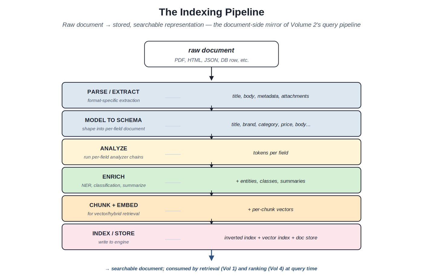
Indexing is the discipline of preparing documents for retrieval. The work happens before any query is issued and runs again whenever documents change. Documents arrive from many sources (databases, content management systems, web crawls, file imports, real-time event streams) in many formats (HTML, PDF, JSON, structured database rows, unstructured text). The indexing pipeline transforms them into a uniform searchable representation: per-field text with appropriate tokenization, structured attributes for filtering, embeddings for semantic retrieval, metadata for ranking signals.
Raw document → parsed and modeled → analyzed → enriched → chunked and embedded → stored. The document-side mirror of Volume 2's query-side pipeline.
The pipeline's position in the broader search architecture. Volume 1 Chapter 1 introduced the search architecture as two pipelines: the query-time pipeline (query understanding, retrieval, ranking, presentation) and the index-time pipeline (parsing, analysis, enrichment, storage). This volume covers the latter. The output of indexing is the corpus that retrieval operates against; the quality of indexing directly determines what retrieval can find and what ranking can score.
The asymmetry that justifies investment. Index-time work happens once per document; query-time work happens once per query. For a typical production system with millions of documents and thousands of queries per second, the per-document amortization makes index-time work cheap relative to query-time work. Ten seconds of additional indexing per document is essentially free at query time — the documents are already in the index when queries arrive. Two milliseconds of additional query-time work, multiplied by every query, is a substantial production cost. The asymmetry favors doing as much work as makes sense at index time.
Where indexing investment pays. Document schemas that support the query patterns the team actually sees. Enrichment that adds structure to unstructured content. Chunking strategies that align with how users formulate queries. Embedding strategies that capture what matters for the workload. Index management that supports schema evolution without downtime. Each of these compounds: better schemas enable better retrieval, which enables better ranking, which produces better outcomes. Teams that under-invest in indexing typically find themselves unable to fix retrieval and ranking problems because the indexing didn't produce the signals those stages would need.
Where indexing investment fails. Schemas that try to support every conceivable query — the over-engineering produces complex indices that are slow to build, expensive to store, and hard to maintain. Enrichment pipelines that add fields no downstream stage uses — the cost without the value. Embedding strategies that embed everything indiscriminately — dilution that produces worse retrieval than focused embedding. Index management without monitoring — silent drift that the team discovers only when queries start failing. The discipline of indexing well includes the discipline of stopping when each addition stops paying off.
Chapter 2. Document Modeling and Schema Design
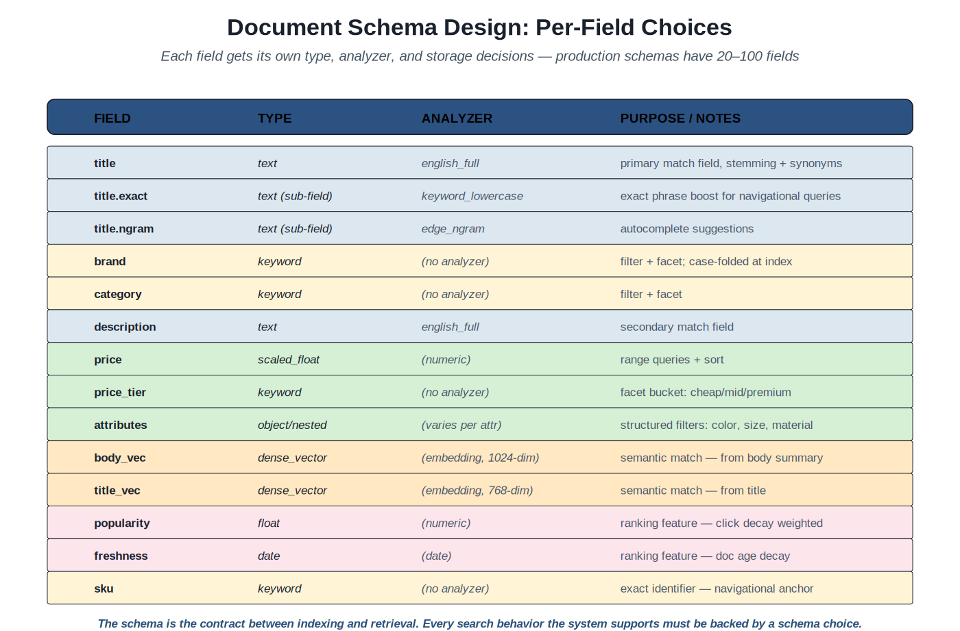
The document schema is the contract between indexing and everything downstream. Every search behavior the system supports must be backed by a schema choice: a field designed to support that behavior, with the right type, analyzer, and storage decisions. Schemas designed without thought to query patterns produce search experiences that no amount of ranking work can fully fix; schemas designed with the patterns in mind produce search experiences where retrieval, ranking, and UX can each do their work well.
Per-field choices: type, analyzer, purpose. Production schemas typically have 20–100 fields supporting different match behaviors and ranking signals.
The field as primary unit. Search engines (Lucene-based and otherwise) organize documents as collections of named fields. Each field has a type (text, keyword, numeric, date, boolean, vector), an analyzer (which determines how text is tokenized for matching), and storage decisions (stored for retrieval, indexed for matching, doc_values for sorting and faceting). The field-level choices are the schema; getting them right is the discipline.
Type choices. Text fields are tokenized and matched lexically with an analyzer. Keyword fields are stored as single tokens without analysis (good for filtering, faceting, and exact match). Numeric fields support range queries and sorting. Date fields support date-range queries and time-based ranking signals. Vector fields support dense retrieval (Volume 1 Section B). Each type fits specific query patterns; choosing the wrong type for a field forces awkward workarounds at query time.
Sub-field patterns. The same underlying content often needs multiple match modes. A product title needs: stemmed lexical match for general queries ("running shoes" matches a title containing "run" after stemming); exact phrase match for navigational queries ("air max 270" should match the exact phrase as a strong boost); edge n-grams for autocomplete (typing "nik" should suggest "nike"). The sub-field pattern (title, title.exact, title.ngram) provides three field representations from one source content, each with its own analyzer, all kept in sync automatically by the indexing engine. Production schemas use sub-fields heavily; the pattern is foundational.
Analyzer assignment. Each field gets an analyzer that determines how its text is tokenized for matching. The analyzer is per-field: title might use english_full (stemming + synonyms); brand might use keyword_lowercase (no tokenization, just case normalization for matching brand names exactly); description might use english_minimal (stemming without synonyms, since description text shouldn't generate as many synonym matches). The choice depends on how the field will be matched; aligning analyzer with intended match behavior prevents many production bugs.
Storage decisions. Stored fields are retrievable (can be displayed in results); indexed fields are matchable (can be queried). Most fields are both, but the distinction matters for fields that are matchable but not display-needed (a stemmed-and-synonymed match field) or display-needed but not matchable (a pre-rendered HTML snippet stored only for display). doc_values determines whether the field is available for sorting and faceting; without doc_values, you can match the field but can't sort or aggregate by it. The choices affect index size and performance.
Vector field choices. Vector fields store dense embeddings for semantic retrieval. The choices include: dimension count (typical: 384 for small models, 768 for medium, 1024+ for large); the underlying ANN index structure (HNSW typical); the similarity metric (cosine for normalized vectors, dot product equivalently); whether to use product quantization for storage efficiency. The choices follow the embedding model selection (Chapter 5); changing model means changing dimensionality means changing the field, which means re-indexing all vectors.
Chapter 3. Index-Time Analysis
Volume 2 Section A documented the analyzer chain (CharFilter → Tokenizer → TokenFilter) as it applies to queries. The same chain runs at index time on every document. The pattern is foundational to lexical search; this chapter covers the index-time perspective and the patterns that emerge there.
Symmetric analysis: index and query use the same chain. The most common configuration runs identical analyzer chains at both times. The advantage: tokens produced at index time match tokens produced at query time, so the inverted index works as expected. A document indexed with the title "Running Shoes" produces tokens [run, shoe]; a query for "ran", analyzed by the same chain, produces token [run]; the inverted index returns the matching document. The symmetry is the design intent of Lucene-based engines and the default operational pattern.
Asymmetric analysis: deliberately different chains. Some patterns use deliberately asymmetric chains. Edge n-gram indexing (produce edge n-grams at index time) with keyword query (no analysis on the query side) supports prefix matching: "nik" matches indexed n-grams [n, ni, nik] of "nike". Synonym expansion at index time (expand the document into all synonym variants when indexing) with no synonym handling at query time (the variants are already in the index) saves query-time work at the cost of index size. The asymmetry is intentional and should be documented; accidental asymmetry is a bug.
Multi-field analysis. The same content often needs to support multiple match modes through multi-field analysis. Index the title into three different fields with three different analyzers: title (stemmed and synonymed), title.exact (case-folded keyword), title.ngram (edge n-grams). The fields share source content but have independent analyzer chains; queries can match against any combination. Production e-commerce schemas commonly have 3–5 sub-fields per important text field; the pattern produces flexibility at the cost of index size.
Language-aware indexing. Multi-language corpora need careful index-time analysis. Options: detect language at index time and apply language-specific analyzers per document (works when language is identifiable, supports per-language stemming and stop words); index multilingual content with a universal analyzer (works for many cases but loses language-specific behavior); index the same content into multiple language-specific fields (title.en, title.fr, title.es) and route queries to the appropriate field based on detected query language. Each pattern has its place; the choice depends on the language distribution and the importance of each language.
Index-time validation. The analyzer chain runs on every document, so analyzer bugs produce indexing failures or worse, silent degradation. Production deployments validate: test the analyzer chain against representative content before deploying schema changes; monitor token counts per field over time (a sudden drop in token count for a field signals an analyzer regression); compare query-time analysis with index-time analysis to ensure symmetry. The validation discipline is part of the broader operations practice that Volume 6 will cover.
Chapter 4. Document Enrichment
Raw documents arrive in many forms, often without the structure that production search needs. A product description is unstructured prose; the brand, category, attributes, target audience are all implicit. An article is body text plus some metadata; the topics, named entities, summary, and sentiment are all latent. Enrichment is the discipline of extracting structured signals from raw content at index time, making them available as fields that retrieval and ranking can use.
The enrichment categories. Named entity recognition at index time: identify entities in the document text (brands, products, locations, people, dates) and store them as structured fields. The work mirrors Volume 2 Section E (query-time NER) but operates on documents; the entity inventories should match between index time and query time so that query entities can match document entities. Classification: assign documents to categories (product categories for e-commerce; topic categories for content). Summarization: generate condensed representations of long documents for display, embedding, or ranking. Attribute extraction: extract specific structured values (price, color, size, material) from semi-structured content. Quality scoring: compute per-document quality scores (completeness, freshness, authority) for use as ranking signals.
Classical vs LLM-based enrichment. Classical NLP methods (spaCy, Stanford NER, custom-trained models) handle enrichment with low latency and predictable cost. They work well for standard entity types and well-defined classification tasks. LLM-based enrichment handles unusual cases that classical methods struggle with: extracting specific attributes from natural-language descriptions; summarizing in domain-specific ways; classifying into nuanced taxonomies. The trade-off is cost: LLM enrichment at index time costs per-document API calls; for large corpora, the costs are non-trivial. Production patterns typically combine: classical methods for the bulk of enrichment; LLM enrichment selectively for the cases that justify the cost.
Incremental enrichment. Enrichment doesn't have to happen all at once. Production patterns: bootstrap with cheap enrichment (rules, classical NER) to get the system live quickly; add LLM-based enrichment selectively for high-value content or specific query classes that need it; backfill the LLM enrichment for older content as resources allow. The incremental pattern lets the team get value early and improve over time rather than waiting for full enrichment before launching.
Enrichment validation. Enriched fields need validation: how accurate is the extraction? Production deployments typically: hold out a labeled sample (manually verified) for accuracy measurement; track per-field extraction rates over time (a sudden drop signals upstream model or data issues); compare enrichment output across pipeline changes via diff and spot-check. The validation discipline overlaps with Volume 5 evaluation methodology applied to indexing pipeline outputs rather than to retrieval outcomes.
The cost-value question. Every enriched field has cost (extraction at index time, storage in the index, complexity in the schema) and value (improved retrieval and ranking from the signal). The discipline is asking the question explicitly: does this field add enough value to justify its cost? Production teams accumulate enrichment fields that look plausible but don't actually contribute to downstream outcomes; periodic field-value audits (which fields are actually used by retrieval and ranking? which have observable downstream impact?) prevent enrichment bloat.
Chapter 5. Chunking and Embedding Strategies
Vector retrieval (Volume 1 Section B) operates on document embeddings. For short documents, the entire document can be embedded as a single vector. For long documents — articles, manuals, books, complex product pages — the document must be broken into chunks, each embedded separately. The chunking strategy substantially affects retrieval quality; the embedding strategy (what to embed, with which model) substantially affects retrieval quality further. Together, chunking and embedding are the most consequential indexing decisions for vector and hybrid retrieval systems.
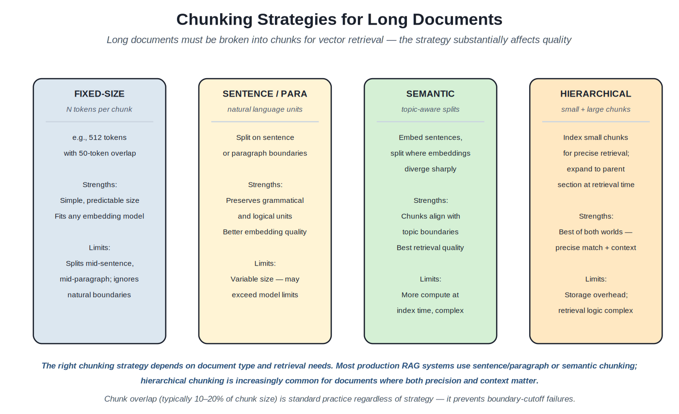
Four chunking strategies with different trade-offs. Hierarchical chunking is the modern production default for documents where both precision and context matter.
Why chunking matters. A long document embedded as a single vector dilutes meaning — the vector represents an average of many topics. A query about one of the topics produces a similarity score lower than the score from a focused chunk about that topic alone. Concretely: embedding a 50-page technical manual into one vector and then querying about a specific topic on page 30 produces a worse match than embedding each section separately and matching against the relevant section. Chunking is the mechanism that produces focused embeddings; the strategy is how the chunking is done.
Fixed-size chunking. Split the document into chunks of N tokens with optional overlap (typical: 512 tokens with 50-token overlap). The simplest strategy: predictable chunk size, fits any embedding model's input limits, no semantic analysis needed. The limit: splits mid-sentence or mid-paragraph, breaking logical units and producing chunks that may miss context. Fixed-size chunking is the default in many RAG frameworks; it works but rarely produces the best quality.
Sentence and paragraph chunking. Split on natural language boundaries: sentences (smallest unit), paragraphs (mid-sized), sections (largest). The strategy preserves logical units within chunks. The limit: variable chunk sizes — some paragraphs are short, some are long, and chunks may exceed embedding model input limits. Production patterns: split by paragraph; if a paragraph exceeds the limit, recursively split by sentence; concatenate small sentences/paragraphs into chunks up to the size limit. The result is chunks that respect natural boundaries while staying within model limits.
Semantic chunking. Embed sentences individually; compute pairwise similarity between adjacent sentences; split where similarity drops below a threshold. The strategy produces chunks that align with topic boundaries within the document. The result is the highest-quality chunks for retrieval. The cost: additional compute at index time (embedding every sentence to determine boundaries) and complexity in the indexing pipeline. Semantic chunking has emerged as a strong production pattern through 2024–2026, especially for technical and educational content.
Hierarchical chunking. Index small chunks (sentences or short paragraphs) for precise retrieval; at retrieval time, also retrieve the parent section or document. The pattern provides both precision (small chunks match queries well) and context (the larger unit provides surrounding context for ranking or for downstream LLM consumption). Storage overhead is higher (multiple chunk levels per document), but retrieval quality benefits substantially. Hierarchical chunking is increasingly the production default for RAG systems where context matters.
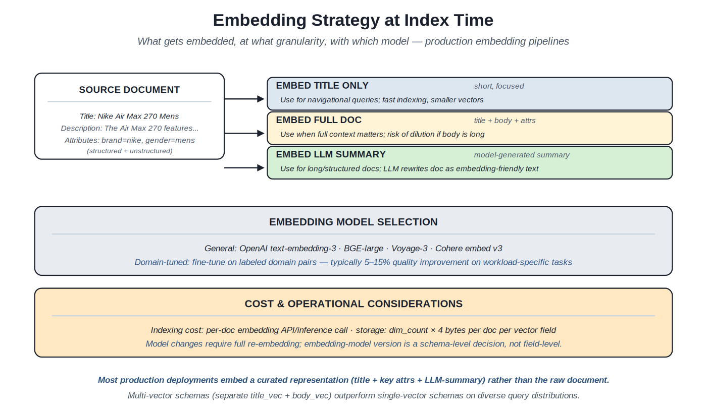
What to embed and with which model. Multi-vector schemas (separate title_vec + body_vec) and curated representations (LLM summaries) typically outperform single-vector full-document embeddings.
What to embed. The choice is less obvious than it appears. Embedding the title alone gives fast indexing, small vectors, and strong navigational-query matching but misses body content. Embedding the full document (or full chunk) captures everything but risks dilution if the body has many tangentially-related concepts. Embedding an LLM-generated summary produces a focused representation that captures what matters most while leaving out incidental detail. Production deployments often use multiple embedding fields: title_vec for navigational matching, body_vec for body-based matching, summary_vec for high-level semantic matching.
Embedding model selection. General-purpose models (OpenAI text-embedding-3, BGE-large, Voyage-3, Cohere embed v3) work for many use cases. Domain-tuned models (fine-tuned on labeled domain-specific pairs) typically produce 5–15% quality improvement over off-the-shelf models on workload-specific tasks. The MTEB leaderboard and BEIR benchmark provide comparison points; production evaluation on the actual workload (Volume 5 Section B) is essential before committing to a model.
Operational considerations. Embedding model selection is a schema-level decision — changing models requires re-embedding the entire corpus, which can be expensive and time-consuming. Embedding API/inference cost at index time accumulates: for large corpora, batched embedding processing is essential to keep costs manageable. Storage costs scale with vector dimensions (1024-dim vectors are roughly 4 KB each at float32; quantization to int8 reduces this to 1 KB at modest quality loss). The operational discipline includes choosing the model carefully, budgeting embedding costs, and planning re-embedding migrations when model upgrades are needed.
Part 2 — The Substrates
Eight sections cover the patterns and methods of indexing and document engineering. Each section opens with a short essay on what its patterns share. Representative patterns appear in the Fowler-style template with code examples for the central methods.
Sections at a glance
- Section A — Document modeling and field design
- Section B — Index-time analyzer chains
- Section C — Enrichment patterns
- Section D — Chunking strategies
- Section E — Embedding strategies
- Section F — Index management (updates, reindexing, versioning)
- Section G — Multi-modal indexing
- Section H — Discovery and resources
Section A — Document modeling and field design
Per-field type decisions, analyzer assignment, sub-field patterns
The schema is the contract between indexing and retrieval. Every search behavior the system supports must be backed by a schema choice; without it, queries can't access the signals they need. The patterns in this section formalize the schema design discipline: how to choose field types, how to design sub-fields, how to keep the schema maintainable as the workload evolves.
Production schema design with sub-fields and multi-mode matching #
Source: Elasticsearch / OpenSearch / Solr schema documentation; Grainger, AI-Powered Search; production methodology at major search teams
Classification — The pattern for designing document schemas that support diverse query patterns through deliberate per-field decisions and sub-field patterns.
Design a document schema where each field's type, analyzer, and storage decisions support the specific query behaviors the system needs to handle, using sub-field patterns to support multiple match modes from a single source content.
Default schemas (one analyzer per field, one match mode per field) produce search experiences that can't handle the variety of query patterns production traffic includes. Navigational queries want exact phrase match; informational queries want stemmed match; autocomplete wants prefix match; faceted browsing wants keyword-style filtering. A schema with one analyzer per field forces compromises: aggressive stemming helps informational queries but hurts navigational ones; conservative analysis helps navigational queries but misses informational matches. The sub-field pattern resolves this by indexing the same content multiple ways with different analyzers; queries can target the appropriate sub-field per match mode.
The field as primary unit. Documents are collections of named fields; each field has a type, analyzer, and storage decisions. The choice of field structure determines what queries can do: a single text field with one analyzer supports one match behavior; multiple sub-fields with different analyzers support multiple match behaviors.
Type choices. Text fields are tokenized and matched lexically (supports phrase queries, multi-word matching, scoring with BM25). Keyword fields store the entire value as one token (supports exact match, filtering, sorting, faceting). Numeric fields (integer, long, float, double, scaled_float) support range queries and sorting. Date fields support time-based queries and decay functions. Boolean fields are filters. Vector fields support dense retrieval (Volume 1 Section B). Geo fields support spatial queries. The choice fits the queries; mismatched types force expensive workarounds.
Sub-field patterns. The pattern of indexing one source content into multiple field variants. The most common: text field with analyzer for general matching; .exact sub-field with keyword analyzer for exact match boost; .ngram sub-field with edge n-gram for autocomplete. The sub-fields share source content; Elasticsearch and OpenSearch handle the multi-field indexing automatically when the schema declares the sub-fields. Queries can target individual sub-fields or boost across multiple sub-fields with appropriate weights.
Analyzer assignment. Per-field analyzer choice depends on intended match behavior. Text fields for natural language: english_full (stemming + synonyms + ASCII fold) for general body text; english_minimal (stemming only) for titles where synonyms might over-broaden. Text fields for identifiers: keyword analyzer (no tokenization). Text fields for autocomplete: edge_ngram analyzer. The analyzer assignment matters for every text-typed field; the choice between text and keyword type for a given field is often the most consequential decision.
Storage decisions. Indexed fields are matchable (queries can match them). Stored fields are retrievable (results can display them). doc_values enable sorting and aggregation. Most fields are all three; specific patterns deviate: a vector field is indexed but not stored (the vector is used for retrieval but not displayed); a pre-rendered HTML field is stored but not indexed (it's for display only). The decisions affect index size and performance; reducing storage on fields that don't need it reduces index footprint.
Nested vs object fields. For structured attributes (color, size, material), the choice is between object fields (each attribute as a top-level field: attributes.color, attributes.size, attributes.material) and nested fields (the attribute is a nested object with cross-field relationships preserved). Nested fields are appropriate when the attributes have meaningful relationships (a size and color combination represents one variant); object fields are appropriate when attributes are independent. The choice affects query expressiveness; nested fields support queries like "red AND size 10 on the same variant" that object fields can't.
Vector field design. Vector fields store dense embeddings for semantic retrieval. Decisions: dimension count (matches the embedding model: 384, 768, 1024, 1536, ...); ANN structure (HNSW typical; alternative: IVF for very large indices); similarity metric (cosine for normalized vectors, equivalent to dot product); element type (float32 standard; int8 quantization for storage reduction). Production schemas typically have 2–3 vector fields (title_vec, body_vec, summary_vec) supporting different match modes.
Schema evolution. Schemas change over time as the workload evolves. Adding fields is generally safe (existing documents have null values for new fields). Changing field types or analyzers requires reindexing (Section F covers the patterns). The discipline is designing schemas with foresight — anticipating likely future fields and reserving naming conventions — but accepting that some schema evolution will require operational work.
Every production search system has a schema, whether deliberately designed or default. The pattern applies universally; the question is whether the design is deliberate. Teams that have not validated their schema design typically have known unknowns in their search capability.
Alternatives — schema-less or document-store retrieval for specific use cases where full-text search isn't the goal. The discipline of schema design remains essential for any production search system.
- Elasticsearch mapping documentation (elastic.co)
- OpenSearch mapping documentation
- Solr schema documentation
- Grainger, AI-Powered Search, chapters on schema design
Schema / config
// Elasticsearch production schema with sub-fields and vector fields
PUT /products
{
  "settings": {
    "analysis": {
      "analyzer": {
        "english_full": {
          "type": "custom",
          "tokenizer": "standard",
          "filter": ["lowercase", "asciifolding", "english_stop", "english_stemmer"]
        },
        "keyword_lowercase": {
          "type": "custom",
          "tokenizer": "keyword",
          "filter": ["lowercase"]
        },
        "edge_ngram": {
          "type": "custom",
          "tokenizer": "standard",
          "filter": ["lowercase", "edge_ngram_filter"]
        }
      },
      "filter": {
        "edge_ngram_filter": {
          "type": "edge_ngram",
          "min_gram": 2,
          "max_gram": 15
        }
      }
    }
  },
  "mappings": {
    "properties": {
      "title": {
        "type": "text",
        "analyzer": "english_full",
        "fields": {
          "exact": { "type": "text", "analyzer": "keyword_lowercase" },
          "ngram": { "type": "text", "analyzer": "edge_ngram" }
        }
      },
      "brand": { "type": "keyword" },
      "category": { "type": "keyword" },
      "description": { "type": "text", "analyzer": "english_full" },
      "price": { "type": "scaled_float", "scaling_factor": 100 },
      "price_tier": { "type": "keyword" },
      "attributes": {
        "type": "nested",
        "properties": {
          "name": { "type": "keyword" },
          "value": { "type": "keyword" }
        }
      },
      "title_vec": {
        "type": "dense_vector",
        "dims": 768,
        "index": true,
        "similarity": "cosine"
      },
      "body_vec": {
        "type": "dense_vector",
        "dims": 1024,
        "index": true,
        "similarity": "cosine"
      },
      "popularity": { "type": "float" },
      "freshness": { "type": "date" },
      "sku": { "type": "keyword" },
      "in_stock": { "type": "boolean" }
    }
  }
}
Section B — Index-time analyzer chains
The analyzer chain on the document side; asymmetric chains and multi-field analysis
Volume 2 Section A covered the analyzer chain from the query-side perspective. The same chain runs at index time on every document. This section documents the index-time perspective: how the chain processes documents, when to use asymmetric chains, and how multi-field analysis supports multi-mode matching.
Symmetric and asymmetric index-time analysis #
Source: Apache Lucene; Elasticsearch / OpenSearch / Solr analyzer documentation; production methodology
Classification — Patterns for running analyzer chains at index time, including symmetric (same chain at index and query) and deliberately asymmetric (different chains) configurations.
Apply analyzer chains at index time to produce the tokens that retrieval will match against, with deliberate choices about whether to use the same chain at query time (symmetric) or to use a different chain for specific match behaviors (asymmetric).
The default configuration runs the same analyzer chain at index and query time. This produces predictable behavior but may not produce the optimal match behavior for all query patterns. Specific patterns (autocomplete, synonym expansion, multi-language) benefit from asymmetric chains where index-time and query-time analysis differ deliberately. The discipline is knowing when symmetric is right and when asymmetric is warranted.
Symmetric analysis: the default and most common. Index and query use identical analyzer chains. Documents indexed with the chain produce tokens; queries processed by the same chain produce tokens that match. The configuration is the design intent of Lucene-based engines: the analyzer chain is associated with the field, and is applied automatically at both index time and query time. The team configures one chain per field; the engine handles applying it correctly at both times.
Asymmetric for autocomplete. Edge n-gram indexing with keyword query. At index time: tokenize and produce edge n-grams of the tokens ("nike" → [n, ni, nik, nike]). At query time: use keyword analyzer (no tokenization beyond lowercasing). The user typing "ni" produces query token [ni] which matches the indexed n-gram [ni] from "nike". The pattern supports prefix matching efficiently; without asymmetric chains, prefix matching requires expensive query-time substring operations.
Asymmetric for synonym expansion. Two options. Option 1: expand synonyms at index time (an indexed document containing "sneakers" gets indexed with tokens [sneakers, running, shoes, footwear]). Query time uses no synonym expansion (the variants are already in the index). Index size grows; query time is faster. Option 2: expand synonyms at query time (the indexed document has [sneakers]; query for "shoes" expands to [shoes, sneakers, footwear] which matches). Index stays lean; query time has more work. Production deployments choose based on whether index-side or query-side complexity is preferred.
Multi-field analysis from one source. The same source content indexed multiple times with different analyzers. Schema declares title with sub-fields title.exact and title.ngram; the indexer automatically produces three sets of tokens from each document's title. Queries can match against title (stemmed match), title.exact (exact phrase), or title.ngram (prefix). The pattern is the foundation of multi-mode matching; production schemas use it heavily for high-value text fields.
Language-aware index-time analysis. For multi-language corpora: detect language at index time per document; apply language-specific analyzer based on detection. A document in French gets the french_analyzer; a document in English gets english_analyzer. Tokens produced are language-appropriate. At query time, language detection on the query routes to the appropriate field. The pattern preserves per-language match quality but requires reliable language detection and per-language analyzer configuration.
Index-time validation. Test the analyzer chain against representative content before deploying schema changes. Use the engine's analyze API (Elasticsearch _analyze, Solr analysis tool) to see exactly what tokens a piece of content produces. Compare with expectations; investigate discrepancies. Production deployments typically maintain test suites of representative content with expected token outputs; schema changes that affect tokenization should pass these tests before deployment.
Operational implications. Index-time analyzer choices are persistent: documents are indexed once with the analyzer in effect at that time; subsequent analyzer changes require reindexing to take effect. The persistence means analyzer changes are not lightweight — they trigger reindexing operations (Section F) that have operational cost. The discipline is designing analyzer chains carefully upfront and treating changes as significant decisions.
All lexical search systems use index-time analyzer chains. Specific asymmetric patterns apply where they're justified by use case: edge n-grams for autocomplete; index-time synonym expansion for query-time performance; language-specific analyzers for multilingual content. The default symmetric pattern is correct for most cases; asymmetric patterns are deliberate optimizations.
Alternatives — keyword-only fields (no tokenization) for exact-match-only fields. Pure vector retrieval bypasses the analyzer chain entirely. The analyzer chain remains foundational for the lexical portion of any hybrid system.
- Apache Lucene analyzer documentation
- Elasticsearch / OpenSearch / Solr analyzer documentation
- Production methodology writings on multi-field schema design
Section C — Enrichment patterns
Index-time NER, classification, summarization, and LLM-based attribute extraction
Enrichment turns raw documents into structured ones. The discipline involves identifying what structure would help downstream stages, choosing methods to extract it, and validating that the extraction works. Modern enrichment combines classical NLP methods for the bulk of work with LLM-based methods for cases that justify the cost.
LLM-based attribute extraction at index time #
Source: Production methodology at e-commerce and content platforms; LLM provider documentation; Pradeep et al. on LLM-based document processing
Classification — Index-time enrichment using LLMs to extract structured attributes, summaries, and classifications from raw documents.
Extract structured signals from raw document content using LLM-based processing at index time, producing fields that retrieval can filter on and ranking can use as features.
Raw documents contain structured information implicitly that classical NLP methods can't reliably extract. A product description in natural language may mention the material, target use case, age recommendation, care instructions, and many other attributes — each as part of the prose rather than as labeled fields. Classical NER catches named entities (brands, locations) but misses domain-specific attributes that require contextual interpretation. LLM-based extraction handles these cases: the model reads the description, understands what's being communicated, and outputs structured fields.
The pattern. For each document at index time: send the document content to an LLM with a structured extraction prompt; parse the LLM's JSON response; store the extracted fields as part of the indexed document. The fields become available for filtering, faceting, and ranking just like manually-curated structured fields would be.
Prompt design. The extraction prompt should specify exactly what fields to extract, with type guidance ("return null if not specified", "extract as ISO date if possible", "one of [casual, formal, athletic]"). Few-shot examples in the prompt substantially improve extraction quality; production prompts typically include 2–5 worked examples. The prompt should produce well-defined JSON output; tool/function-calling APIs (Anthropic's tool use, OpenAI's function calling) provide stronger structure guarantees than freeform JSON generation.
Model selection. Smaller, cheaper models (Claude Haiku, GPT-4o-mini, Gemini Flash) handle straightforward extraction with low cost. Larger models (Claude Opus, GPT-4) are warranted for complex extraction or when accuracy is critical. The trade-off depends on document complexity and cost sensitivity. Production deployments often use smaller models by default and route specific document types to larger models when justified.
Batch processing. Extraction at index time can be batched aggressively. For large initial indexing runs, send batches of documents through the LLM API in parallel; production deployments routinely process thousands of documents per minute through batched extraction. The Anthropic batch API and similar batch endpoints offer cost discounts (50% off) for non-real-time processing, making large extraction runs more economical.
Validation. LLM extraction quality varies; production deployments need validation. Hold out a labeled sample (manually verified) and measure extraction accuracy per field. Track extraction rates over time (fraction of documents where each field was successfully extracted); a sudden drop signals upstream issues. Spot-check extracted values against source documents for high-value fields.
Failure handling. LLM calls can fail or produce malformed output. Production extraction pipelines handle failures: retry with backoff for transient API errors; fall back to null/missing values for repeated failures; alert on failure rates above thresholds; maintain a queue of failed documents for re-processing. The pipeline should not let LLM failures block the entire indexing process.
Cost management. LLM extraction at index time has per-document cost; for large corpora the total cost matters. Strategies: process only high-value content with LLM extraction (use cheaper methods for the long tail); extract only the high-value fields with LLM (use rules or classical NLP for simple fields); cache extraction results aggressively so re-indexing doesn't pay the cost again; use batch APIs when latency permits.
Incremental enrichment. New documents arrive continuously; the pipeline must process them. Production patterns: process new documents through the LLM extraction pipeline as they arrive, with appropriate parallelism; for updated documents, only re-extract if the changed fields affect extracted output (avoid unnecessary re-extraction of unchanged content). The discipline keeps the index current without over-processing.
E-commerce search where products have unstructured descriptions that contain extractable structured information (material, occasion, age, fit, style). Content platforms where articles need topic extraction, sentiment analysis, or summarization. Enterprise search where documents have implicit structure (jurisdiction, date, case type, document type) that explicit fields would benefit from. Use cases where classical NLP methods can't reach the extraction quality the downstream stages need.
Alternatives — classical NLP for entities and standard classification (cheaper, faster, predictable). Rule-based extraction for simple cases. Manual annotation for the highest-value content where neither classical nor LLM methods are sufficient. Production deployments typically combine all three: rules for the simplest cases, classical NLP for standard cases, LLM for cases needing contextual understanding.
- Anthropic Claude documentation on tool use and batch API
- OpenAI function calling documentation
- Production methodology writings on LLM-based document processing
- Pradeep, Nogueira, Lin on LLM-based document processing
Code
# LLM-based attribute extraction at index time with Claude
import anthropic
import json
from typing import Optional

client = anthropic.Anthropic()

# Define the extraction tool/schema - tool use gives structural guarantees
EXTRACTION_TOOL = {
"name": "extract_product_attributes",
"description": "Extract structured product attributes from the description",
"input_schema": {
"type": "object",
"properties": {
"material": {
"type": ["string", "null"],
"description": "Primary material (e.g., 'leather', 'mesh', 'rubber'). Null if not specified."
},
"occasion": {
"type": ["string", "null"],
"enum": ["casual", "formal", "athletic", "work", "outdoor", None],
"description": "Primary use occasion. Null if unclear."
},
"target_gender": {
"type": ["string", "null"],
"enum": ["mens", "womens", "unisex", "kids", None]
},
"features": {
"type": "array",
"items": {"type": "string"},
"description": "Notable product features mentioned (e.g., 'waterproof', 'memory foam insole')"
},
"summary": {
"type": "string",
"description": "One-sentence product summary suitable for semantic embedding"
}
},
"required": ["summary"]
}
}

def extract_attributes(title: str, description: str) -> dict:
"""Extract structured attributes from a product description."""
prompt = f"""Extract structured attributes from this product:

Title: {title}
Description: {description}

Use the extract_product_attributes tool. Be conservative --- only fill fields where the description provides clear evidence; use null otherwise."""
response = client.messages.create(
model="claude-haiku-4-5-20251001", # Haiku for speed and cost
max_tokens=1024,
tools=[EXTRACTION_TOOL],
tool_choice={"type": "tool", "name": "extract_product_attributes"},
messages=[{"role": "user", "content": prompt}]
)
# Tool use guarantees structured output
for block in response.content:
if block.type == "tool_use":
return block.input
return {}

# Batch processing pattern for initial indexing
def enrich_documents_batch(docs: list[dict]) -> list[dict]:
"""Enrich a batch of documents. In production, use the Anthropic batch API for cost savings."""
enriched = []
for doc in docs:
try:
attrs = extract_attributes(doc["title"], doc["description"])
enriched.append({
**doc,
"material": attrs.get("material"),
"occasion": attrs.get("occasion"),
"target_gender": attrs.get("target_gender"),
"features": attrs.get("features", []),
"llm_summary": attrs.get("summary"), # source for body_vec embedding
})
except Exception as e:
# Log and continue; don't block indexing on enrichment failures
print(f"Extraction failed for {doc.get('id')}: {e}")
enriched.append(doc)
return enriched

# Validation pattern: check extraction quality against held-out labeled sample
def validate_extraction(labeled_sample: list[dict]) -> dict:
"""Compare LLM extraction against manually labeled gold sample."""
results = {"material": {"correct": 0, "total": 0},
"occasion": {"correct": 0, "total": 0}}
for doc in labeled_sample:
extracted = extract_attributes(doc["title"], doc["description"])
for field in results:
if doc.get(f"gold_{field}") is not None:
results[field]["total"] += 1
if extracted.get(field) == doc[f"gold_{field}"]:
results[field]["correct"] += 1
return {
field: r["correct"] / r["total"] if r["total"] > 0 else None
for field, r in results.items()
}
Section D — Chunking strategies
Fixed-size, sentence/paragraph, semantic, and hierarchical chunking for vector retrieval
Long documents must be broken into chunks for vector retrieval. The chunking strategy substantially affects retrieval quality — chunks that align with natural boundaries and topic structures produce better matches than arbitrary fixed-size splits. The patterns in this section document the strategies and the operational details that make them work.
Chunking strategies for production vector retrieval #
Source: RAG framework documentation (LangChain, LlamaIndex); production methodology in 2023–2026 RAG deployments; semantic chunking literature
Classification — Methods for breaking long documents into retrieval-sized chunks for embedding and vector retrieval.
Choose a chunking strategy appropriate to the document type and retrieval needs, producing chunks that maximize retrieval quality at acceptable index size and indexing cost.
A long document embedded as a single vector dilutes meaning. A query about a specific topic on page 30 of a 50-page document produces a poor match against the document's pooled embedding. Chunking addresses this by producing focused embeddings: each chunk represents a coherent piece of content, embedded separately, indexed as a separate retrievable unit. The strategy is how the chunking is done; the choice affects retrieval quality substantially.
Fixed-size chunking. Split the document into chunks of N tokens with overlap. Typical configuration: 512 tokens per chunk with 50-token overlap (overlap prevents matches at chunk boundaries from being lost). The strategy is simple, predictable, and fits any embedding model's input limits. The downside: splits ignore natural boundaries, breaking sentences and paragraphs mid-stream. Despite this limitation, fixed-size chunking remains popular for its simplicity and is the default in many RAG frameworks.
Sentence and paragraph chunking. Split on natural language boundaries. Process: identify sentence/paragraph boundaries; group sentences or paragraphs into chunks up to a size limit (e.g., 512 tokens); maintain overlap between chunks. The result is chunks that respect natural units — better embedding quality than fixed-size, but with variable sizes. For documents where paragraphs are well-formed (articles, manuals, books), this strategy often produces better retrieval than fixed-size.
Semantic chunking. Identify topic boundaries within the document and split there. The standard algorithm: embed each sentence individually; compute pairwise cosine similarity between adjacent sentences; identify sharp similarity drops as topic boundaries; group sentences between boundaries into chunks. The result is chunks that align with semantic topics; embedding quality is high. The cost is additional compute at index time (embedding every sentence to determine boundaries). Semantic chunking is the modern production default for complex documents where the additional compute is justified.
Hierarchical chunking. Index multiple chunk levels: small chunks (e.g., individual sentences or short paragraphs) for precise retrieval; larger chunks (e.g., sections) or full documents accessible at retrieval time for context. At retrieval time: search the small chunks; for each match, fetch the parent section or full document as context. The pattern provides precision (small chunks match well) and context (the parent provides surrounding information that helps ranking or downstream LLM consumption). Storage overhead is higher — chunks at multiple levels — but retrieval quality benefits.
Chunk overlap. All chunking strategies typically include overlap between adjacent chunks (10–20% of chunk size is typical). The overlap ensures that content near chunk boundaries isn't lost: a query that matches content split across two chunks can match either chunk because the boundary content appears in both. Without overlap, boundary content can be effectively invisible to retrieval. The overlap costs index size proportionally; the quality benefit usually justifies it.
Chunk metadata. Each chunk should carry metadata that retrieval can use: the source document ID (so retrieval can group chunks by document or fetch the parent document); the chunk position within the document (for ordering and context); the source section/header (for displaying "from section X" in results); the chunk size (for adapting downstream processing). The metadata is part of the indexed representation and consumed at retrieval time.
Document type considerations. Different document types benefit from different strategies. Code documentation: chunk by function or class. API documentation: chunk by endpoint. Books: chunk by chapter or section. Technical articles: chunk by section, with semantic chunking within sections. Product descriptions: typically short enough not to need chunking. The strategy should fit the structure of the documents being indexed.
Chunk size tuning. The optimal chunk size depends on the workload. Small chunks (256 tokens): precise retrieval but may lack context. Large chunks (1024 tokens): more context but may dilute meaning. Most production deployments find optimal sizes between 384 and 768 tokens. The tuning is empirical: test multiple sizes against the workload's queries and pick the size with the best retrieval metrics (NDCG@K, MRR; Volume 5 covers).
Any production system doing vector retrieval on long documents. RAG pipelines (agentic AI Volume 10). Enterprise search over documentation. Content discovery over articles or research papers. The chunking strategy is foundational to retrieval quality; the choice matters.
Alternatives — no chunking for short documents (entire document fits in one embedding). Document-level retrieval with separate ranking-time context extraction for cases where retrieval can be at document level but generation needs specific spans. The chunking decision depends on document type and retrieval needs.
- LangChain documentation on text splitters
- LlamaIndex documentation on chunking
- Production methodology writings on RAG chunking (2023–2026)
Code
# Semantic chunking implementation - the modern production default
import numpy as np
from sentence_transformers import SentenceTransformer
from typing import List, Dict

model = SentenceTransformer('all-mpnet-base-v2')

def semantic_chunk(
text: str,
similarity_threshold: float = 0.5,
min_chunk_tokens: int = 128,
max_chunk_tokens: int = 768,
) -> List[Dict]:
"""Split text into chunks at semantic boundaries.
Algorithm:
1. Split into sentences
2. Embed each sentence
3. Compute similarity between adjacent sentences
4. Split where similarity drops below threshold (topic boundary)
5. Respect min/max chunk size constraints
"""
# Split into sentences (production: use spaCy or nltk for robust splitting)
import re
sentences = re.split(r'(?<=[.!?])\s+', text.strip())
if len(sentences) < 2:
return [{"text": text, "start_sent": 0, "end_sent": 0}]
# Embed all sentences
embeddings = model.encode(sentences, normalize_embeddings=True)
# Compute pairwise similarity between adjacent sentences
similarities = [
float(np.dot(embeddings[i], embeddings[i+1]))
for i in range(len(sentences) - 1)
]
# Identify boundary candidates: similarity dips
chunks = []
current_chunk_start = 0
current_token_count = len(sentences[0].split())
for i, sim in enumerate(similarities):
next_sent = sentences[i + 1]
next_tokens = len(next_sent.split())
# Force-split if max size would be exceeded
if current_token_count + next_tokens > max_chunk_tokens:
chunks.append({
"text": " ".join(sentences[current_chunk_start:i + 1]),
"start_sent": current_chunk_start,
"end_sent": i,
})
current_chunk_start = i + 1
current_token_count = next_tokens
continue
# Topic-boundary split if similarity dips and chunk is big enough
if sim < similarity_threshold and current_token_count >= min_chunk_tokens:
chunks.append({
"text": " ".join(sentences[current_chunk_start:i + 1]),
"start_sent": current_chunk_start,
"end_sent": i,
})
current_chunk_start = i + 1
current_token_count = next_tokens
else:
current_token_count += next_tokens
# Final chunk
if current_chunk_start < len(sentences):
chunks.append({
"text": " ".join(sentences[current_chunk_start:]),
"start_sent": current_chunk_start,
"end_sent": len(sentences) - 1,
})
return chunks

# Hierarchical chunking: small chunks for retrieval, larger context available
def hierarchical_chunk(doc: dict) -> dict:
"""Produce small chunks linked to their parent section."""
sections = parse_into_sections(doc["text"]) # implementation-specific
all_small_chunks = []
for section_idx, section in enumerate(sections):
small_chunks = semantic_chunk(section["text"], max_chunk_tokens=256)
for chunk in small_chunks:
all_small_chunks.append({
**chunk,
"doc_id": doc["id"],
"section_idx": section_idx,
"section_text": section["text"], # available for context at retrieval time
"section_title": section["title"],
})
return {
"doc_id": doc["id"],
"chunks": all_small_chunks,
"sections": sections,
}
Section E — Embedding strategies
What to embed, with which model, with what update cadence
Chapter 5 of Part 1 covered embedding strategy at a conceptual level. This section makes the discipline concrete: how to choose what to embed, how to combine structured and unstructured content for embedding, how to manage embedding model versioning at production scale.
Production embedding strategies and multi-vector schemas #
Source: OpenAI, Cohere, Voyage AI, BGE embedding model documentation; production methodology in modern RAG and semantic search deployments
Classification — Patterns for selecting embedding models, designing what to embed, and managing embeddings as the schema evolves.
Choose embedding model, content representation, and field structure to produce high-quality vector representations that retrieval can use effectively across the diverse queries the system handles.
Embedding a document is more than running text through a model. What text to embed, at what granularity, with which model, in how many fields — each decision affects retrieval quality. Defaults (embed the body, one vector field, off-the-shelf model) work but often miss substantial quality gains available through deliberate design. The patterns documented here capture the production discipline that emerges from teams who have invested in embedding strategy.
What to embed: the choice. The simplest choice is to embed the full document text. The pattern works but produces dilution for long or multi-topic documents — the embedding represents an average of concepts. Better patterns: embed a curated representation. Title-only embedding for navigational matching. Title + key attributes (brand, category, top 5 features) for focused matching. LLM-generated summary for documents where the original text is verbose or structurally complex. Multi-vector schemas (separate title_vec and body_vec) for different match modes.
Multi-vector schemas. A schema with multiple vector fields per document, each capturing a different aspect. Common pattern: title_vec for navigational matches (typically 768-dim, focused on title content); body_vec for descriptive matches (1024-dim, broader context); summary_vec for high-level semantic matches (generated from LLM summary). Queries match against multiple vector fields with different weights; the LTR model (Vol 4 Section B) learns the appropriate weighting per query class. Multi-vector schemas substantially outperform single-vector schemas on diverse query distributions.
Embedding model selection. General-purpose models cover many cases: OpenAI text-embedding-3-large (1536 dims, strong general quality, commercial API); BGE-large (1024 dims, open source, self-hostable); Voyage AI voyage-3 (1024 dims, high quality on RAG tasks, commercial API); Cohere embed v3 (1024 dims, multilingual). The MTEB leaderboard provides comparative quality data; the BEIR benchmark provides retrieval-specific evaluation. Production evaluation on the actual workload (Volume 5 Section B) is essential before committing.
Domain fine-tuning. Off-the-shelf embedding models work but domain-tuned models typically produce 5–15% quality improvement on workload-specific tasks. The training process: collect labeled relevance pairs (query, positive document, hard negative document) from production logs or judgment lists; fine-tune the base model with contrastive loss; evaluate the tuned model on held-out evaluation queries. The investment is non-trivial but produces durable quality gains; production teams with mature search practice typically invest in this.
LLM-generated content for embedding. Embedding model quality depends on the input text quality. Documents with verbose or poorly-structured content produce lower-quality embeddings; documents with clean, focused content produce higher-quality embeddings. The pattern: use an LLM at index time to generate a clean summary or representation; embed the LLM output rather than the raw document. The LLM acts as content normalizer; the embedding model receives high-quality input. Production deployments routinely combine LLM-generated representations with raw-content fields, providing multiple embedding paths.
Embedding model versioning. The embedding model is a schema-level decision — changing models means re-embedding the entire corpus. Production discipline: treat embedding model selection as a deliberate schema decision; record the model version with the index metadata; plan model upgrades as substantial migrations (Section F covers); maintain compatibility windows during transitions (run two models in parallel during migration). The discipline prevents accidental incompatibilities.
Cost management. Embedding API/inference cost at index time accumulates. Strategies: batch processing for cost efficiency (most providers offer batch discounts of 50%+); selective embedding (only embed content above a length threshold; for very short content like product titles, embedding may not add value over lexical matching); incremental updates (only re-embed when content changes substantively, not on every metadata update); fine-tuned smaller models (a tuned smaller model can match an off-the-shelf larger model at lower per-document cost). Production deployments typically combine multiple strategies to keep embedding costs manageable.
Quality monitoring. Production embedding pipelines need quality monitoring. Track: embedding generation rate (how many docs per hour are being embedded); embedding generation failures (API errors, timeouts); embedding quality metrics on held-out evaluation queries (NDCG@K from vector retrieval over time). Sudden changes in these signals indicate issues with the embedding pipeline that need investigation. The monitoring discipline is part of operations (Volume 6 planned).
Any production search system using vector retrieval. RAG pipelines. Hybrid retrieval systems where vector is one component. Cross-modal search where embeddings bridge modalities (Section G). The embedding strategy decisions affect quality substantially; deliberate design beats defaults.
Alternatives — lexical-only retrieval (Volume 1 Section A) for cases where semantic matching isn't needed. Pre-computed similarity tables for very small corpora where ANN structures aren't justified. Most modern production search uses vector embeddings somewhere; the strategy is how they're used.
- OpenAI embedding documentation (platform.openai.com)
- Cohere embed documentation (docs.cohere.com)
- Voyage AI embed documentation
- BGE / FlagEmbedding documentation (huggingface.co/BAAI)
- MTEB leaderboard (huggingface.co/spaces/mteb/leaderboard)
- BEIR benchmark (github.com/beir-cellar/beir)
Section F — Index management
Partial updates, blue/green reindexing, embedding-model migrations
Indices change. Schemas evolve, embedding models upgrade, content updates continuously. The patterns in this section cover how to manage these changes without downtime: when to apply partial updates, how to execute blue/green reindexing, how to migrate embedding models. The discipline is essential for production search; without it, schema evolution requires downtime or accepts data inconsistency.
Blue/green reindexing with index aliases #
Source: Elasticsearch / OpenSearch alias documentation; production methodology for zero-downtime schema evolution
Classification — Pattern for executing schema or analyzer changes without downtime by building the new index alongside the live one and atomically switching.
Evolve indices (schema changes, analyzer changes, embedding model changes) without downtime by building a new index version alongside the live one, reindexing all data, and atomically switching queries to point at the new version.
Schema and analyzer changes require reindexing — existing documents indexed under the old configuration won't work correctly with the new configuration. Naive approaches (delete and recreate the index, with downtime; or in-place mutation, which most engines don't support) either accept downtime or aren't possible. The blue/green pattern allows zero-downtime migration by building the new state alongside the old and switching atomically.
The alias primitive. Elasticsearch and OpenSearch (and Solr in different form) support index aliases: named pointers that can target an index. Applications query against the alias (e.g., "products"); the alias resolves to a specific underlying index (e.g., "products_v2024_05_19"). The alias can be atomically reassigned to point at a different underlying index. Queries that arrive during reassignment see a consistent state — they hit either the old or new index, never partial state.
The blue/green workflow. Step 1: build the new index with the new schema or configuration ("products_v2024_05_20"). Step 2: reindex all documents from the old index to the new index using the engine's reindex API (or a custom pipeline that re-reads source data and re-emits to the new index). Step 3: validate the new index has all expected content with the new schema applied. Step 4: atomically swap the alias from old to new. Step 5: keep the old index for some grace period (in case rollback is needed) then drop it.
Reindexing cost. The reindex step is the expensive one. For native reindexing (Elasticsearch _reindex API), cost is proportional to document count and complexity of any transformations. For custom reindexing (re-read source data, re-process, re-emit), cost includes data source access. Either way, reindex of a large corpus takes hours to days. The cost is non-trivial; teams should budget for it as part of any major schema change.
Validation gates. Before swapping the alias, validate the new index: document count matches expected (no docs lost in reindex); spot-check specific documents for correct schema application (the new analyzer produces expected tokens); run a representative query set against the new index and compare results to the old index (changes are expected, but they should be the expected changes); for substantial changes, A/B test the new index with a small traffic fraction before full swap.
Rollback capability. The pattern provides rollback for free: if the new index has issues, swap the alias back to the old index. The rollback is atomic and fast. Keep the old index for a grace period (typically days to weeks after the swap, depending on confidence in the new index and the cost of keeping it). Eventually drop the old index to free storage.
Embedding model migrations. The most expensive blue/green case. Changing embedding models requires re-embedding every document with the new model — substantial LLM API or inference cost. Production migrations: budget the embedding cost explicitly; use batch APIs (50% discount available); execute the embedding in parallel during off-peak hours; maintain old index until new index is validated; consider phased migration (re-embed high-traffic content first, then long-tail).
Partial updates vs reindex. For changes that affect a single field's value (price change, popularity refresh, inventory update), partial updates (the engine's update API) work in-place — no reindex needed. For changes to field types or analyzers, partial updates aren't possible — the field's on-disk representation depends on the original schema. Knowing which changes need reindex and which don't is essential operational knowledge.
Incremental indexing patterns. Production indices receive ongoing updates: new documents, document updates, document deletes. During blue/green reindexing, both the old and new indices must continue receiving updates. The discipline: the indexing pipeline writes to both indices during reindex (dual-write pattern); after swap, the old index can stop receiving updates. The dual-write requirement adds operational complexity but is essential for keeping the new index current during the migration.
Every production indexing pipeline that does any meaningful indexing should support blue/green or equivalent zero-downtime patterns. Schema evolution is part of any maturing system; without zero-downtime capability, schema changes accumulate as deferred work that never gets done.
Alternatives — in-place mutation where the engine supports it (rare for substantive changes). Brief planned downtime for non-critical systems. Application-level dual-source reads during transition (more complex than alias swapping but provides similar capability for engines without alias support).
- Elasticsearch alias documentation (elastic.co)
- OpenSearch alias documentation
- Elasticsearch _reindex API documentation
- Production methodology writings on zero-downtime schema migration
Schema / config
// Elasticsearch blue/green reindexing pattern with aliases

// Step 1: Create new index with new schema
PUT /products_v2024_05_20
{
  "settings": { /* new settings */ },
  "mappings": { /* new mappings */ }
}

// Step 2: Reindex from old to new (Elasticsearch _reindex API)
POST /_reindex?wait_for_completion=false
{
  "source": { "index": "products_v2024_05_19" },
  "dest": { "index": "products_v2024_05_20" },
  "script": {
    "source": "/* optional inline transformation during reindex */"
  }
}
// Returns a task ID; monitor with: GET /_tasks/<task_id>

// Step 3: Validate new index
GET /products_v2024_05_20/_count // doc count should match old
GET /products_v2024_05_20/_search // representative queries return expected results
GET /products_v2024_05_20/_analyze // analyzer behavior matches expectations
{
"field": "title",
"text": "Sample content for testing"
}

// Step 4: Atomic alias swap - this is the critical step
POST /_aliases
{
  "actions": [
    { "remove": { "index": "products_v2024_05_19", "alias": "products" }},
    { "add": { "index": "products_v2024_05_20", "alias": "products" }}
  ]
}
// Queries against alias "products" now hit the new index atomically
// Either before or after - never partial

// Step 5: Keep old index for grace period, then drop
// After confidence period (typically days to weeks):
DELETE /products_v2024_05_19

// During reindexing: dual-write to BOTH indices to keep them in sync
// Application code:
// def index_document(doc):
// es.index(index="products", document=doc) // via alias - goes to old
// if migration_in_progress:
// es.index(index="products_v2024_05_20", document=doc) // explicit new
// After alias swap, the old index can be safely retired

// For embedding model migrations, the reindex step includes re-embedding:
// The custom pipeline reads each doc from old, re-embeds with new model, writes to new index
Section G — Multi-modal indexing
Image, audio, and video embeddings alongside text
Modern search increasingly spans multiple modalities: text alongside images for product search; text alongside audio for podcast search; text alongside video for video discovery. The patterns in this section cover the indexing-side of multi-modal search: how to extract and store cross-modal embeddings that retrieval can use to match across modalities.
Multi-modal embedding for cross-modal search #
Source: CLIP (Radford et al., 2021); production methodology for multi-modal search; modern multi-modal embedding models
Classification — Pattern for indexing documents with embeddings from multiple modalities, supporting cross-modal retrieval (text-to-image, image-to-text, audio-to-text).
Index documents that combine text, images, audio, or video by extracting embeddings from each modality and storing them as separate vector fields, supporting retrieval that matches across modalities.
E-commerce products have text descriptions and product images; users sometimes search with text ("red running shoes") and sometimes with images ("shoes that look like this"). Content discovery includes text articles, podcast episodes (audio), and video clips; users want to find content across modalities. Pure text indexing misses the visual and audio signals; pure modality-specific indexing fragments the search experience. Multi-modal indexing addresses this by extracting embeddings from each modality and combining them in retrieval.
Cross-modal embedding models. The key technology is models that embed multiple modalities into a shared vector space. CLIP (OpenAI, 2021) was the breakthrough: text and images embedded into the same space, such that a text query and a matching image produce similar vectors. Modern alternatives: OpenCLIP (open-source CLIP variants), SigLIP (Google's improved CLIP), Cohere's multi-modal embeddings, BGE-M3 (multilingual + multi-modal). The models produce embeddings that support cross-modal queries: text against images, images against images, images against text.
Indexing pipeline. For each document with multiple modalities: extract embeddings from each modality using the appropriate model (or unified multi-modal model). For products: text embedding from title and description; image embedding from product photo. For articles with images: text embedding from body; image embeddings from inline images. Store each embedding as a separate vector field. The schema supports retrieval against any modality.
Storage and indexing. Each modality's embedding becomes a vector field in the document schema (Section A pattern). For a product: title_vec (text), description_vec (text), image_vec (visual). Each vector field is independently indexed with appropriate ANN structure. Retrieval can match against text fields with text queries, against image fields with image queries (after embedding the query image into the same space), or against both with hybrid queries.
Modality-specific extraction. Different modalities have different extraction patterns. Images: process through a vision model (CLIP or similar) to produce a single embedding per image; for documents with multiple images, decide whether to store one embedding per image (more storage, finer-grained matching) or pool images into one document-level embedding (less storage, coarser matching). Audio: process through an audio model (CLAP or similar) or first transcribe to text and embed the transcript. Video: process keyframes through a vision model and/or audio track through an audio/text pipeline.
Cross-modal retrieval. The retrieval-side pattern: a text query is embedded with the text-side of the multi-modal model; the embedding is used in ANN search against the image_vec field; results are products whose images match the text query semantically. The pattern works because the model embedded text and images into the same space — nearest neighbors in the shared space are semantically related across modalities. The query at retrieval time names which fields to search; multi-field queries (search both text and image_vec) provide additional flexibility.
Embedding model trade-offs. CLIP and successors are general-purpose; they work for many use cases but aren't optimized for specific domains. Domain-fine-tuned CLIP models (fashion-CLIP for clothing, FoodCLIP for food, BioCLIP for biology) produce substantially better results on their domains. Production deployments often fine-tune CLIP on labeled domain pairs (image, text-description) to capture domain-specific semantics.
Operational considerations. Image processing at index time has computational cost (vision model inference per image); for large catalogs the cost matters. Storage: image embeddings are typically 512–1024 dim, similar to text embeddings, with similar storage characteristics. Update frequency: image embeddings don't need to be recomputed unless the image or model changes; text embeddings should be recomputed when content changes substantively. The pipeline complexity is higher than text-only indexing but well-established patterns exist.
E-commerce search where product images are central to the user experience (fashion, home decor, art). Content discovery across modalities (Spotify, YouTube). Visual search applications ("find products like this"). Domain-specific multi-modal search (medical imaging plus text, satellite imagery plus text descriptions). Cross-modal search increasingly common as multi-modal LLMs and embeddings mature.
Alternatives — text-only indexing where images are tangential. Separate single-modality search engines that don't share a vector space (older pattern that doesn't support cross-modal queries). The multi-modal pattern is the modern default where multiple modalities are part of the corpus.
- Radford et al., "Learning Transferable Visual Models From Natural Language Supervision" (CLIP, 2021)
- OpenCLIP repository (github.com/mlfoundations/open_clip)
- SigLIP paper and implementations
- Cohere multi-modal embedding documentation
- Production methodology writings on multi-modal search at major e-commerce companies
Section H — Discovery and resources
Where to track indexing discipline as the field continues to evolve
Indexing and document engineering draws from IR, NLP, ML, and increasingly from RAG and multi-modal research. The discipline continues to evolve; staying current requires tracking multiple sources.
Resources for tracking indexing and document engineering discipline #
Source: Multiple academic, practitioner, and tool sources
Classification — Sources for staying current on indexing and document engineering practice.
Provide pointers to the active sources of indexing knowledge across IR, NLP, ML, RAG, and production practice.
Indexing intersects multiple disciplines: classical IR for index structures; NLP for analyzer chains; ML for embeddings; RAG for chunking strategies; multi-modal research for cross-modal indexing. Production teams need engagement with each.
Foundational texts. Manning, Raghavan, Schütze, Introduction to Information Retrieval (free online) — chapters 2 (text processing), 4 (index construction), 5 (index compression). Grainger, AI-Powered Search (Manning, 2024) — strong production-focused chapters on indexing for modern search including vector and hybrid patterns. Turnbull and Berryman, Relevant Search (Manning, 2016) — practical lexical-search indexing in depth.
Academic conferences. SIGIR for IR-side methods including index structures and analysis. ACL/EMNLP for NLP methods including NER and classification used in enrichment. NeurIPS/ICML/ICLR for embedding methods and multi-modal models. The CIKM, WSDM venues for IR systems work including indexing infrastructure.
Industry venues. Haystack Conference covers indexing alongside other search topics. Berlin Buzzwords for IR and data engineering. RAG-focused conferences emerging through 2024–2026 (the RAG Summit, NeurIPS RAG workshops).
Practitioner writing. Daniel Tunkelang on indexing strategy. OpenSource Connections on lexical and hybrid indexing. Search team blogs at Etsy, Wayfair, Spotify, GitHub publish substantial indexing case studies periodically. The agentic AI series' Volume 10 (RAG) covers RAG-specific indexing patterns from a different angle.
Tools and libraries. Apache Lucene (foundational; underlies Elasticsearch/OpenSearch/Solr). Vector databases: Pinecone, Weaviate, Qdrant, Chroma, Milvus. Embedding pipelines: LangChain text splitters, LlamaIndex chunking utilities, sentence-transformers for self-hosted embedding. Multi-modal: OpenCLIP, SigLIP, transformers (Hugging Face) for vision models. RAG frameworks: LangChain, LlamaIndex, Haystack (deepset).
Embedding model registries and benchmarks. Hugging Face Model Hub for pretrained models including embeddings. MTEB leaderboard for embedding model comparison. BEIR benchmark for retrieval-specific evaluation. The leaderboards inform model selection; production evaluation on the actual workload remains essential.
Communities. Hugging Face forums for embedding model discussion. LangChain and LlamaIndex Discord/Slack for RAG indexing patterns. Relevancy Engineering Slack for search-specific indexing discussion. Vector database vendor communities (Pinecone, Weaviate, Qdrant Discord servers).
Emerging areas. Long-context embedding models (handling longer documents per embedding). Multi-vector models (multiple vectors per document for finer-grained matching, ColBERT-style at the embedding side). Mult-modal embedding extending beyond image-text to audio, video, structured data. Sparse embeddings (SPLADE family) blurring the lexical/semantic boundary. The frontier is active; tracking proceedings and major model releases catches most developments.
Search engineers building or maintaining indexing pipelines. Engineers transitioning into search from data engineering or ML engineering. Continuous education as the field evolves. Reference for specific indexing decisions where current knowledge needs supplementing.
Alternatives — specialized consulting for high-stakes engagements. Internal documentation for teams with mature practice. The combination of external tracking and internal knowledge is the working pattern.
- Manning et al., Introduction to Information Retrieval (free online)
- Grainger, AI-Powered Search (2024)
- Apache Lucene documentation
- SIGIR, Haystack, Berlin Buzzwords proceedings
- LangChain, LlamaIndex, Haystack RAG framework documentation
- MTEB and BEIR benchmarks
- Relevancy Engineering Slack
Appendix A — Pattern Reference Table
Cross-reference of the indexing patterns covered in this volume, what each provides, and when to use each.
| Pattern | Provides | When to use | Section |
|---|---|---|---|
| Schema with sub-fields | Multi-mode matching from one source | All production schemas | Section A |
| Symmetric analyzer chains | Consistent index/query tokens | Default for lexical match | Section B |
| Asymmetric analyzer chains | Special match behaviors | Autocomplete, index-time synonyms | Section B |
| LLM-based attribute extraction | Structured signals from unstructured | E-commerce, content platforms | Section C |
| Fixed-size chunking | Simple, predictable size | Simple RAG, framework default | Section D |
| Semantic chunking | Topic-aligned chunks | Best retrieval quality | Section D |
| Hierarchical chunking | Precision + context | RAG where both matter | Section D |
| Multi-vector schemas | Multiple match modes via vectors | Diverse query distributions | Section E |
| Embedding model versioning | Manage embedding migrations | Production at scale | Section E |
| Blue/green reindexing | Zero-downtime evolution | Any maturing system | Section F |
| Multi-modal embedding (CLIP) | Cross-modal retrieval | Visual + text search | Section G |
Appendix B — The Search Engineering Series
This catalog is Volume 3 of the Search Engineering Series. The current state of the series:
- Volume 1 — The Search Patterns Catalog (delivered) — query-time architectural patterns.
- Volume 2 — The Query Understanding Catalog (delivered) — the methods that produce structured query signals.
- Volume 3 — The Indexing and Document Engineering Catalog (this volume) — the document-side preparation that retrieval depends on.
- Volume 4 — The Ranking and Relevance Catalog (delivered) — scoring functions, learning to rank, neural rerankers.
- Volume 5 — The Search Evaluation Catalog (delivered) — metrics, judgment collection, online evaluation.
- Volume 6 — The Search Operations Catalog (planned) — tuning workflows, query log analysis, regression investigation.
- Volume 7 — The Search UX Patterns Catalog (planned) — autocomplete, facets, snippets, did-you-mean.
- Volume 8 — The Search Platforms Survey (planned) — Elasticsearch, OpenSearch, Solr, Coveo, Algolia, Vespa.
With Volume 3 delivered, the series has five of its planned core volumes (1, 2, 3, 4, 5). These five together cover the complete query-time and index-time pipelines plus the methodology for measuring outcomes. The remaining priority volume is 6 (Search Operations) for day-to-day tuning workflow. Volumes 7 and 8 round out the broader coverage but are less essential than 6 for production practice.
Appendix C — The Five-Volume Foundation
With Volume 3 delivered, the Search Engineering Series has its five-volume foundation. Volume 1 establishes architectural vocabulary; Volume 2 covers the query-side processing; Volume 3 covers the document-side preparation; Volume 4 covers the ranking methods; Volume 5 covers the evaluation methodology. The five volumes together provide structural reference for end-to-end production search engineering practice.
Touchpoints between volumes. The analyzer chain (Volume 2 Section A, Volume 3 Section B) is the same machinery applied at query time and at index time — the symmetry is the design intent. The query understanding outputs (Volume 2 Sections D, E, F) need to align with the document enrichment outputs (Volume 3 Section C) so that entity-aware queries can match entity-enriched documents. The chunking and embedding strategies (Volume 3 Sections D, E) determine what retrieval (Volume 1 Sections B, C) can do. The schema decisions (Volume 3 Section A) determine which ranking features (Volume 4 Section C) are available. Volume 5's evaluation discipline catches regressions across all of the above; effective debugging often traces from a Volume 5 alert back through Volumes 1–4 to identify the cause.
Use as a working library. The five volumes function as a working reference library for production search engineering. A typical client engagement: Volume 5 establishes the evaluation baseline; Volume 1 frames the architectural assessment; investigation typically surfaces issues across Volumes 2, 3, and 4; recommendations span all four production volumes plus the evaluation discipline. The library structure mirrors how practitioners actually work — across pipeline stages, not within one stage at a time.
Reading order recommendations. For a practitioner new to search engineering: Volume 1 first (architectural vocabulary), Volume 5 second (measurement discipline), Volume 2 third (query side), Volume 3 fourth (document side, this volume), Volume 4 last (ranking methods). The order grounds in architecture and measurement before diving into the specific subdisciplines. For an experienced practitioner: any volume can be read standalone for its focus; the cross-references make integration straightforward.
What's missing. Operations (Volume 6) is the most pressing gap — the day-to-day tuning workflow that integrates the methodologies from the other volumes into practice. UX patterns (Volume 7) covers presentation that this volume's indexing decisions ultimately enable. Platforms Survey (Volume 8) compares the major platforms' implementations of the patterns. The five core volumes are sufficient for most production work; the additional volumes add depth in specific areas.
Appendix D — Discovery and Standards
Resources for tracking indexing discipline (consolidated from Section H):
- Foundational texts: Manning et al., Introduction to Information Retrieval (free online); Grainger, AI-Powered Search (Manning, 2024); Turnbull and Berryman, Relevant Search (Manning, 2016).
- Academic conferences: SIGIR (IR-side); ACL/EMNLP (NLP-side); NeurIPS/ICML/ICLR (embedding/multi-modal); CIKM/WSDM (IR systems).
- Industry venues: Haystack Conference, Berlin Buzzwords.
- Practitioner writing: Daniel Tunkelang, OpenSource Connections, search team blogs.
- Tools and libraries: Apache Lucene; vector databases (Pinecone, Weaviate, Qdrant, Chroma, Milvus); RAG frameworks (LangChain, LlamaIndex, Haystack); multi-modal (OpenCLIP, SigLIP).
- Embedding model resources: Hugging Face Model Hub; MTEB leaderboard; BEIR benchmark.
- Communities: Relevancy Engineering Slack; LangChain/LlamaIndex Discord; vector database vendor communities.
Three practical recommendations. First, Apache Lucene documentation is dense but worth reading carefully — it's the foundation underlying Elasticsearch, OpenSearch, and Solr, and understanding Lucene's analyzer chain and indexing model prevents many production issues. Second, the BEIR benchmark and MTEB leaderboard provide objective comparison points for retrieval and embedding choices; periodic evaluation of your system's methods against these benchmarks tells you where you stand vs. the field. Third, indexing-side improvements often produce the largest production quality gains because so many teams under-invest in this discipline — the marginal value of indexing investment is high precisely because the baseline is so low.
Appendix E — Omissions
This catalog covers about 10 patterns across 8 sections — the scope of a structural volume on indexing. The wider discipline includes much that isn't covered here:
- Streaming and near-real-time indexing in depth (Kafka-based pipelines, change data capture, low-latency document updates). Operational topic; deserves dedicated treatment.
- Index compression and storage optimization (column compression, posting list compression, vector quantization in depth). Specialized topic; vendor documentation covers.
- Distributed indexing architectures (shard design, replication, cross-region indexing). Engine-specific; vendor docs cover well.
- Index lifecycle management at scale (hot-warm-cold tiering, automated rollover, retention policies). Operations-adjacent; future Volume 6.
- Source data integration patterns (CDC from databases, file-system crawlers, message queue ingestion). Bridges to data engineering.
- Domain-specific schema patterns (legal documents, medical records, code, scientific papers). Each domain has its own conventions.
- Sparse embedding models (SPLADE family) for hybrid lexical-semantic indexing. Emerging area worth a dedicated section in a future revision.
- Graph-based indexing (knowledge graph storage alongside text). Bridges to knowledge graph engineering.
- Fine-tuning embedding models in depth (training data construction, contrastive learning, hard negative mining). ML methodology; sentence-transformers documentation covers.
- Embedding model evaluation methodology beyond MTEB (domain-specific evaluation, production drift detection). Operations topic.
Appendix F — The Document-Side Mirror
Volume 3 is the document-side mirror of Volume 2. Both volumes cover the same underlying machinery from different angles: Volume 2 from the query-side, Volume 3 from the document-side. The mirror relationship is intentional — the analyzer chain that processes queries at query time is the same chain that processes documents at index time, with the same configuration; the entity recognition that identifies entities in queries should match the entity recognition that identifies entities in documents; the embedding models that embed queries should embed documents into the same vector space.
Why two volumes rather than one. The query-side and document-side have different operational concerns even though they share machinery. Query-side processing happens in the query path with latency constraints; document-side processing happens at index time with throughput constraints. Query-side processing operates on user-typed strings with their characteristic variations; document-side processing operates on diverse source content with its characteristic structure. The two volumes can be read together for the symmetric view, or independently when the focus is one side.
Where the volumes diverge. Volume 2 covers patterns that have no document-side equivalent: spell correction (queries get misspelled; documents don't), query rewriting (queries get reformulated; documents stay as-is), intent classification (queries have intent; documents have content). Volume 3 covers patterns that have no query-side equivalent: schema design (documents have schemas; queries don't), chunking (long documents are chunked; queries rarely need chunking), index management (indices need versioning; queries are ephemeral). The mirror is partial; each volume documents both the shared machinery and the side-specific concerns.
Consulting application. The two volumes together provide complete reference for the most underdeveloped area of production search practice. Many search engagements involve issues that span both sides — query understanding outputs that don't align with document enrichment outputs, embedding models on the query side that don't match the index side, analyzer chains that work for queries but not for the indexed documents. Having both volumes available lets the practitioner work across the symmetry deliberately rather than ad-hoc.
The next volume. With Volumes 1, 2, 3, 4, and 5 in place, the series has its five-volume foundation. Volume 6 (Search Operations) is the natural next — the day-to-day workflow that integrates the methodologies from the other volumes into practice. Operations is where indexing and query-side decisions meet production reality: zero-result queries that reveal indexing gaps; ranking regressions that trace back to analyzer changes; embedding-model migrations that need careful execution. The operational discipline ties the technical disciplines together.
— End of The Indexing and Document Engineering Catalog (Volume 3) —
— Volume 3 of the Search Engineering Series —